Time Series Forecasting with Python – Part 1 (Simple Linear Regression)

In this series of posts, I’ll be covering how to approach time series forecasting in python in detail. We will start with the basics and build on top of it. All posts will contain a practice example attached as a GitHub Gist. You can either read the post or watch the explainer Youtube video below.

# Loading Libraries
import numpy as np
import pandas as pd
import seaborn as sns

We will be using a simple linear regression to predict the outcome of the number of flights in the month of May. The data is taken from seaborn datasets.

sns.set_theme()
flights = sns.load_dataset("flights")
flights.head()

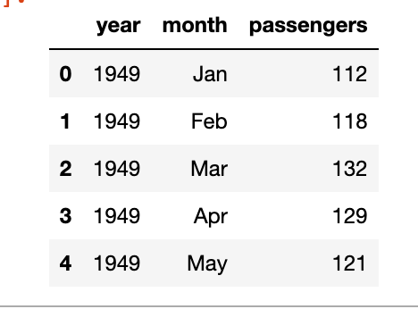
As you can see we’ve the year, the month and the number of passengers, as a dummy example we will focus on the number of passengers in the month of May, below is the plot of year vs passengers.

We can clearly see a pattern here and can build a simple linear regression model to predict the number of passengers in the month of May in future years. The model will be like y = slope * feature + intercept. The feature, in this case, will be the number of passengers but shifted by 1 year. Meaning the number of passengers in the year 1949 will be the feature for the year 1950 and so on.

df = flights[flights.month == 'May'][['year', 'passengers']]
df['lag_1'] = df['passengers'].shift(1)
df.dropna(inplace = True)

Now we have the feature, let’s build the model-

import statsmodels.api as sm
y = df['passengers']
x = df['lag_1']
model = sm.OLS(y, sm.add_constant(x))
results = model.fit()
b, m = results.params

Looking at the results

OLS Regression Results                            
==============================================================================
Dep. Variable:             passengers   R-squared:                       0.969
Model:                            OLS   Adj. R-squared:                  0.965
Method:                 Least Squares   F-statistic:                     279.4
Date:                Fri, 20 Jan 2023   Prob (F-statistic):           4.39e-08
Time:                        17:52:21   Log-Likelihood:                -47.674
No. Observations:                  11   AIC:                             99.35
Df Residuals:                       9   BIC:                             100.1
Df Model:                           1                                         
Covariance Type:            nonrobust                                         
==============================================================================
                 coef    std err          t      P>|t|      [0.025      0.975]
------------------------------------------------------------------------------
const         13.5750     17.394      0.780      0.455     -25.773      52.923
lag_1          1.0723      0.064     16.716      0.000       0.927       1.217
==============================================================================
Omnibus:                        2.131   Durbin-Watson:                   2.985
Prob(Omnibus):                  0.345   Jarque-Bera (JB):                1.039
Skew:                          -0.365   Prob(JB):                        0.595
Kurtosis:                       1.683   Cond. No.                         767.
==============================================================================

We can see that the p-value of the feature is significant, the intercept is not so significant, and the R-squared value is 0.97 which is very good. Of course, this is a dummy example so the values will be good.

df['prediction'] = df['lag_1']*m + b
sns.lineplot(x='year', y='value', hue='variable', 
             data=pd.melt(df, ['year']))

The notebook is uploaded as a GitHub Gist –