Huber Loss – Loss function to use in Regression when dealing with Outliers

Huber loss, also known as smooth L1 loss, is a loss function commonly used in regression problems, particularly in machine learning tasks involving regression tasks. It is a modified version of the Mean Absolute Error (MAE) and Mean Squared Error (MSE) loss functions, which combines the best properties of both.

Below are some advantages of Huber Loss –

1. Robustness to outliers: One of the main advantages of Huber loss is its ability to handle outliers effectively. Unlike Mean Squared Error (MSE), which heavily penalizes large errors due to its quadratic nature, Huber loss transitions to a linear behaviour for larger errors. This property reduces the impact of outliers and makes the loss function more robust in the presence of noisy data.
2. Differentiability: Huber loss is differentiable at all points, including the transition point between the quadratic and linear regions. This differentiability is essential when using gradient-based optimization algorithms, such as Stochastic Gradient Descent (SGD), to update the model parameters during training. The continuous and differentiable nature of the loss function enables efficient optimization.
3. The balance between L1 and L2 loss: Huber loss combines the benefits of both Mean Absolute Error (MAE) and MSE loss functions. For small errors, it behaves similarly to MSE (quadratic), which helps the model converge faster during training. On the other hand, for larger errors, it behaves like MAE (linear), which reduces the impact of outliers.
4. Smoother optimization landscape: The transition from quadratic to linear behaviour in Huber loss results in a smoother optimization landscape compared to MSE. This can prevent issues related to gradient explosions and vanishing gradients, which may occur in certain cases with MSE.
5. Efficient optimization: Due to its smoother nature and better handling of outliers, Huber loss can lead to faster convergence during model training. It enables more stable and efficient optimization, especially when dealing with complex and noisy datasets.
6. User-defined threshold: The parameter δ in Huber loss allows users to control the sensitivity of the loss function to errors. By adjusting δ, practitioners can customize the loss function to match the specific characteristics of their dataset, making it more adaptable to different regression tasks.
7. Wide applicability: Huber loss can be applied to a variety of regression problems across different domains, including finance, image processing, natural language processing, and more. Its versatility and robustness make it a popular choice in many real-world applications.

While there are also some disadvantages of using this loss function –

1. Hyperparameter tuning: The Huber loss function depends on the user-defined threshold parameter, δ. Selecting an appropriate value for δ is crucial, as it determines when the loss transitions from quadratic (MSE-like) to linear (MAE-like) behaviour. Finding the optimal δ value can be challenging and may require experimentation or cross-validation, making the model development process more complex.
2. Task-specific performance: Although Huber loss is more robust to outliers compared to MSE, it might not be the best choice for all regression tasks. The choice of loss function should be task-specific, and in some cases, other loss functions tailored to the specific problem might provide better performance.
3. Less emphasis on smaller errors: The quadratic behavior of Huber loss for small errors means that it might not penalize small errors as much as the pure L1 loss (MAE). In certain cases, especially in noiseless datasets, the added robustness to outliers might come at the cost of slightly reduced accuracy in predicting smaller errors.

Let’s see Huber Regression in Action and see how it is different compared to Linear Regression

import numpy as np
from sklearn.linear_model import HuberRegressor, LinearRegression
from sklearn.datasets import make_regression
import seaborn as sns
sns.set_theme()
rng = np.random.RandomState(0)
X, y, coef = make_regression(n_samples=200, n_features=2, noise=4.0, coef=True, random_state=0)

#Adding outliers
X[:4] = rng.uniform(10, 20, (4, 2))
y[:4] = rng.uniform(10, 20, 4)

#plotting the data 

sns.scatterplot(x = X[:,1], y = y)
sns.scatterplot(x = X[:,0], y = y)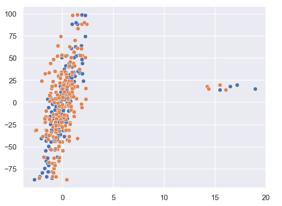

As we can see from our data plotted that there are a few outliers in this.
Let us see how Huber Regression and Linear Regression perform.

huber = HuberRegressor().fit(X, y)

lr = LinearRegression()
lr.fit(X,y)

print(f'True coefficients are {coef}')
>>>True coefficients are [20.4923687  34.16981149]
print(f'Huber coefficients are {huber.coef_}')
>>>Huber coefficients are [17.79064252 31.01066091]
print(f'Linear coefficients are {lr.coef_}')
>>>Linear coefficients are [-1.92210833  7.02266092]

Here we can see that the Huber coefficients are closer to the true coefficients, let us also visualise this by plotting the line.

# use line_kws to set line label for legend

fig, axes = plt.subplots(nrows=1, ncols=2, figsize=(10, 5))
sns.regplot(x=X[:,1], y=y, color='b', 
 line_kws={'label':"y={0:.1f}x+{1:.1f}".format(huber.coef_[1],huber.intercept_)}, ax = axes[0])
axes[1] = sns.regplot(x=X[:,1], y=y, color='r', 
 line_kws={'label':"y={0:.1f}x+{1:.1f}".format(lr.coef_[1],lr.intercept_)}, ax = axes[1])

In these plots, we can clearly see the effect the outlier has on the regression output between Linear and Huber Regression.