Author: sahaymaniceet

  • Ultimate Guide to Chroma Vector Database: Everything You Need to Know – Part 2

    Ultimate Guide to Chroma Vector Database: Everything You Need to Know – Part 2

    In Part 1, we learned how to create the vector database and add documents to a collection. In this tutorial, we will learn how you can query the collection, upsert documents, delete individual documents and also the collection.

    Querying

    Now you can either peek at the collection, which will return you the first 10 documents in the collection, you can also specify the number of documents to peek at, or you can specify either the metadata or the ID you want to retrieve.

    collection.peek(5) # Returns the top 5 documents
    collection.get(ids=['pdf_chunk_0', 'pdf_chunk_1']) # Returns the documents corresponding to ids mentioned in the list

    You can also query a collection using the where method, where you can specify metadata. For example, in Part 1 we added metadata to each document, where the file name was reasearch_paper. So we can query all documents with the metadata.

    collection.get(where={'file_name': 'reasearch_paper'})

    Another thing you can do is query the most similar documents to an input query. For example, I want to know in the research paper who the authors are, I can get the documents which may contain this information by running –

    collection.query(query_texts=["Who are the authors of the paper ?"], n_results=3)

    Here the query texts are my queries and n_results is the number of similar documents I want for the query. You can specify multiple queries at the same time. In that case, it will return results for each query at the same time.

    Upserting

    Similar to querying, you can upsert providing the IDs. So for example I want to upsert the data in ID pdf_chunk_0, then I’ll run the following –

    collection.upsert(ids=['pdf_chunk_0'], documents=['This is an example of upsertion'])

    Now if I query the document, I should see the above document text instead of the original document. Note that if you provide an ID which is not present, ChromaDB will consider it as an add operation.

    Deleting

    Again you can delete individual documents by either specifying the IDs or using the where method. So in case I want to delete pdf_chunk_0, I can run this – collection.delete(ids = ['pdf_chunk_0']) or if I want to delete all documents containing some metadata, I can run this query – collection.delete(where={"file_name": "research_paper"})

    You can also delete the entire collection by client.delete_collection('research')

    In case you want to reset the client, and you’ve allowed so when creating the persistent client in the setting, you can run client.reset(). Empties and completely resets the database. ⚠️ This is destructive and not reversible.

    Let me know In case you want to learn more about ChromaDB, then I’ll create a guide for advanced users.

  • Ultimate Guide to Chroma Vector Database: Everything You Need to Know – Part 1

    Ultimate Guide to Chroma Vector Database: Everything You Need to Know – Part 1

    In this tutorial, we will walk through how to use Chromadb as your vector database for all your Retrieval-Augmented Generation (RAG) tasks.

    But before that, you need to install Chromadb, if you’re using Python then all you need to do is –

    pip install chromadb

    Now that you’ve installed Chromadb, let’s begin. We will use a PDF file as an example. For the PDF we will be using this research paper, but feel free to use the PDF of your choice.

    The first step is to create a persistent client, i.e., the storage which can be used at multiple places. While creating the client remember to add the setting to allow resetting the client should you require this functionality.

    import chromadb
    
    client = chromadb.PersistentClient(
                path="<path of persistent storage>", settings=chromadb.config.Settings(allow_reset=True)
            )

    Once you’ve a client set up then you can define collections within it. If you use BigQuery or any SQL products, imagine the client being the project and the collection being the dataset. Within the collection, you can store the documents as embeddings. In this example, we will call our collection as “research”. Also, one very important thing to remember is that each collection should have its own embedding function that has to be fixed. The query is also passed as an embedding when you try to search for the most similar documents. So in case you use embedding function X to add the documents and use embedding function Y to query them, then the similarity scores will not be correct, so this is a point to remember. We will be using the OpenAI ttext-embedding-3-small model. Another point to remember is that in a single document, you should only have as many tokens as the embedding function can embed. If say your embedding function is all-MiniLM-L6-v2 from HuggingFace, then the max sequence length that the function can handle is 256, so if you try to vectorise a file with longer context, then it will just clip the document to 256 tokens and embed that. The model from OpenAI has a longer max sequence length, but how much exactly is hard to find.

    # Defining the embedding function
    embedding_func = embedding_functions.OpenAIEmbeddingFunction(api_key=os.environ.get("OPENAI_API_KEY") , 
                                                                 model_name="text-embedding-3-small")
    

    Creating the collection, it’s best practice to specify the embedding function while creating the collection, otherwise, Chromadb uses a default embedding function. Chromadb will use sentence-transformer as a default if no embedding function is supplied.

    Now we will need to add a document to this collection, for this, we will use some helper functions from langchain.

    from langchain.text_splitter import RecursiveCharacterTextSplitter
    from langchain_community.document_loaders import PyPDFLoader
    
    data_path = "./data/2311.04635v1.pdf"
    
    pdf_loader = PyPDFLoader(data_path)
    text_splitter = RecursiveCharacterTextSplitter(
        chunk_size=1000,
        chunk_overlap=50,
        separators=["\n\n", "\n", ". ", " ", ""],
    )
    documents = pdf_loader.load_and_split(text_splitter=text_splitter)

    The PyPDFLoader will help to load the PDF file and the RecursiveCharacterTextSplitter will help in splitting the PDF into chunks. We are using a chunk size of 1000 with an overlap of 50, meaning the chunk sizes will be roughly 1000 tokens with overlapping text of 50 tokens. You can learn more about how the text splitter works here.

    Now that we have our documents loaded, time to add them to the Chromadb collection. Since we’ve specified the embedding function in the collection already, we can simply add the text files as embeddings. You have to specify “ids”, and think of them as table names in SQL, also you can specify metadata for each document, both are useful when you want to upsert or delete documents in the collection.

    collection.add(
                documents=[i.page_content for i in documents],
                ids=[f"pdf_chunk_{i}" for i in range(len(documents))],
                metadatas=
                [
                    {
                        "file_name": "reasearch_paper",
                        "timestamp": datetime.now(timezone.utc).isoformat(),
                    }
                    for _ in documents
                ],
            )

    Here we use the page contents of the loaded documents as documents, since they are text, the collection using its embedding function will automatically convert them as embeddings. In case you already have embeddings, you can directly add them as embeddings. I’ve also specified some ids, these are very rudimentary here for illustration purposes. Also, I’ve specified some metadata for each document. Both of these will be used to query, upsert or delete individual documents from the vector database.

    Read more about how you can upsert documents, query a collection and delete individual documents in Part II of this Ultimate Guide to ChromaDB

  • Deep Cross Networks Explained – An Evolution of Feed Forward Networks

    Deep Learning has revolutionized various sectors lately. One critical component of this revolution is the emergence of the Deep Cross Network (DCN). DCN is a novel type of neural network that significantly deviates from the traditional feed-forward networks to offer more robust and efficient solutions. This article aims to provide an in-depth understanding of the Deep Cross Network, its differences from the traditional feed-forward networks, and the areas of its application.

    Understanding Deep Cross Network (DCN)

    The Deep Cross Network (DCN) is a sophisticated hybrid model that combines the strengths of deep neural networks (DNNs) and feature crossing. It was introduced to handle high-dimensional sparse data more efficiently. It’s a mix of deep learning for non-linear input-output mappings and feature crossing for capturing some form of interaction between the feature dimensions.

    The core idea behind DCN is to apply explicit and efficient feature crossing in an input space. This is done by using a cross network that applies a cross operation on the input features to learn explicit bounded-degree feature interactions, which is then combined with a deep network that models arbitrary interactions.

    How DCN Differs From Feed-Forward Networks

    Feed-forward networks or Multilayer Perceptrons (MLPs) are the simplest type of artificial neural network. In these networks, data moves in one direction—from the input layer, through the hidden layers, and finally to the output layer. There is no looping or cycling back of data.

    DCN, on the other hand, doesn’t strictly adhere to this one-way flow. Instead, it allows the explicit feature crossing, which essentially enables the model to learn certain feature interactions and feed them back into the model. This combination of explicit and bounded-degree feature crossing with deep networks gives DCN its unique strength.

    Another notable difference lies in the complexity and efficiency of the two models. While feed-forward networks can become computationally expensive and complex as they increase in size and depth, DCN manages to handle high-dimension sparse input effectively and efficiently, thanks to its unique architecture.

    Another distinguishing feature is the ability of DCN to model feature interactions. While standard feed-forward networks can struggle to capture intricate feature interactions without substantial depth, DCN excels at learning both low- and high-order feature interactions effectively.

    Applications of Deep Cross Network

    The Deep Cross Network has numerous applications across various domains. Some of the most prevalent are:

    1. Recommendation Systems: DCN can effectively handle high-dimensional data and capture complex feature interactions, making it suitable for recommendation systems. It can model the interactions between users and items efficiently to provide accurate recommendations.
    2. Advertisement Click Prediction: DCN’s ability to capture high-order feature interactions makes it a perfect fit for predicting advertisement clicks. By understanding the intricate relationships between user behavior, ad characteristics, and context, it can predict the likelihood of a user clicking on an ad.
    3. Fraud Detection: In banking and finance, DCN can be used for fraud detection by effectively modeling the complex relationships between various transactions.
    4. Natural Language Processing: DCN can also be applied to various NLP tasks, such as sentiment analysis or text classification, where it can learn effective feature interactions from high-dimensional text data.

    Conclusion

    The Deep Cross Network is a significant breakthrough in the field of deep learning. Its unique combination of deep networks and feature crossing distinguishes it from traditional feed-forward networks and makes it a powerful tool for handling high-dimensional sparse data.

    Let me know in the comments if you want to go over an application of Deep Cross Networks using an example dataset.

  • Embed Documents Using Ollama – OllamaEmbeddings

    You can now create document embeddings using Ollama. Also once these embeddings are created, you can store them on a vector database. You can read this article where I go over how you can do so.

    from langchain_community.embeddings import OllamaEmbeddings
    ollama_emb = OllamaEmbeddings(
    model="mistral",
    )
    r1 = ollama_emb.embed_documents(
    [
    "Alpha is the first letter of Greek alphabet",
    "Beta is the second letter of Greek alphabet",
    "This is a random sentence"
    ]
    )
    r2 = ollama_emb.embed_query(
    "What is the second letter of Greek alphabet"
    )

    Let’s inspect the array shapes-

    print(np.array(r1).shape)
    >>> (3,4096)
    print(np.array(r2).shape)
    >>> (4096,)

    Now we can also find the cosine similarity between the vectors –

    from sklearn.metrics.pairwise import cosine_similarity
    cosine_similarity(np.array(r1), np.array(r2).reshape(1,-1))
    >>>array([[0.62087283],
    [0.65085897],
    [0.36985642]])

    Here we can clearly see that the second document in our 3 reference documents is the closest to our question. Similarly, you can also create embeddings from your text documents and store them and can later query them using Ollama and LangChain.

  • How does ChatGPT remember? LLM Memory Explained.

    In the fascinating world of conversational AI, the ability of systems like ChatGPT to remember and refer back to earlier parts of a conversation is nothing short of magic. But how does this seemingly simple act of recollection work under the hood? Let’s dive into the concept of memory in large language models (LLMs) and uncover the mechanisms that enable these digital conversationalists to keep track of our chats.

    The Essence of Memory in Conversational AI

    Memory in conversational AI systems is about the ability to store and recall information from earlier interactions. This capability is crucial for maintaining the context and coherence of a conversation, allowing the LLM to reference past exchanges and build upon them meaningfully. This also gives the appearance that the LLM has intelligence when in reality they are stateless and have no inbuilt memory.

    LangChain, a framework for building conversational AI applications, highlights the importance of memory in these systems. It distinguishes between two fundamental actions that a memory system needs to support: reading and writing.

    What happens is that the LLM is passed an additional context of memory in addition to your input as a prompt so that it can process the information as if it had all the context from the get-go.

    Building Memory into Conversational Systems

    The development of an effective memory system involves two key design decisions: how the state is stored and how it is queried.

    Storing: The Backbone of Memory

    Underneath any memory system lies a history of all chat interactions. These can range from simple in-memory lists to sophisticated persistent databases. Storage is simple, you can store all past conversations in a database. You can either store them as simple text documents or use a vector database and store them as embeddings.

    Querying: The Brain of Memory

    Storing chat messages is only one part of the equation. The real magic happens in the querying phase, where data structures and algorithms work together to present a view of the message history that is most useful for the current context. This might involve returning the most recent messages, summarizing past interactions, or extracting and focusing on specific entities mentioned in the conversation.

    Practical Implementation with LangChain

    Here we will take a look at one way to store memory using LangChain.

    from langchain.memory import ConversationBufferMemory

    memory = ConversationBufferMemory(memory_key="chat_history", return_messages=True)

    Now you can attach this memory to any LLM chain and it will add the entire previous conversations as context to the LLM after each chain invoke. The advantage of using this kind of memory is that its simple to implement. The disadvantage is that in longer conversations you’re passing more tokens and the input prompt size explodes, meaning slower response and if you’re using paid models like GPT-4, then costs also increase.

    Conclusion

    The ability of systems like ChatGPT to remember past interactions is a cornerstone of effective chatbots. By leveraging sophisticated memory systems, developers can create applications that not only understand the current context but can also draw on previous exchanges to provide more coherent and engaging responses. As we continue to push the boundaries of what conversational AI can achieve, the exploration and enhancement of memory mechanisms will remain a critical area of focus.

  • Build RAG Application Using Ollama

    In this tutorial, we will build a Retrieval Augmented Generation(RAG) Application using Ollama and Langchain. For the vector store, we will be using Chroma, but you are free to use any vector store of your choice.

    There are 4 key steps to building your RAG application –

    1. Load your documents
    2. Add them to the vector store using the embedding function of your choice.
    3. Define your prompt template.
    4. Deinfe your Retrieval Chatbot using the LLM of your choice.

    In case you want the collab notebook, you can click here.

    First we load the required libraries.

    # Loading required libraries
    import os

    from langchain.text_splitter import RecursiveCharacterTextSplitter
    from langchain_community.document_loaders import PyPDFLoader
    from langchain_community.vectorstores import Chroma
    from langchain.chains import RetrievalQA
    from langchain.memory import ConversationSummaryMemory
    from langchain_openai import OpenAIEmbeddings
    from langchain.prompts import PromptTemplate
    from langchain.llms import Ollama

    Then comes step 1 which is to load our documents. Here I’ll be using Elden Ring Wiki PDF, you can just visit the Wikipedia page and download it as a PDF file.

    data_path = "./data/Elden_Ring.pdf"
    text_splitter = RecursiveCharacterTextSplitter(
    chunk_size=2000,
    chunk_overlap=30,
    length_function=len,)

    documents = PyPDFLoader(data_path).load_and_split(text_splitter=text_splitter)

    The next step is to use an embedding function that will convert our text into embeddings. I prefer using OpenAI embeddings, but you can use any embedding function. Using this embedding function we will add our documents to the Chroma vector database.

    embedding_func = OpenAIEmbeddings(api_key=os.environ.get("OPENAI_API_KEY"))
    vectordb = Chroma.from_documents(documents, embedding=embedding_func)

    Moving on, we have to define a prompt template. I’ll be using the mistral model, so its a very basic prompt template that mistral provides.

    template = """<s>[INST] Given the context - {context} </s>[INST] [INST] Answer the following question - {question}[/INST]"""
    pt = PromptTemplate(
    template=template, input_variables=["context", "question"]
    )

    All that is left to do is to define our memory and Retrieval Chatbot using Ollama as the LLM.

    rag = RetrievalQA.from_chain_type(
    llm=Ollama(model="mistral"),
    retriever=vectordb.as_retriever(),
    memory=ConversationSummaryMemory(llm = Ollama(model="mistral")),
    chain_type_kwargs={"prompt": pt, "verbose": True},
    )
    rag.invoke("What is Elden Ring ?")
    >>> {'query': 'What is Elden Ring ?',
    'history': '',
    'result': ' Elden Ring is a 2022 action role-playing game developed by FromSoftware. It was published for PlayStation 4, PlayStation 5, Windows, Xbox One, and Xbox Series X/S. In the game, players control a customizable character on a quest to repair the Elden Ring and become the new Elden Lord. The game is set in an open world, presented through a third-person perspective, and includes several types of weapons and magic spells. Players can traverse the six main areas using their steed Torrent and discover linear hidden dungeons and checkpoints that enable fast travel and attribute improvements. Elden Ring features online multiplayer mode for cooperative play or player-versus-player combat. The game was developed with inspirations from Dark Souls series, and contributions from George R.R. Martin on the narrative and Tsukasa Saitoh, Shoi Miyazawa, Tai Tomisawa, Yuka Kitamura, and Yoshimi Kudo for the original soundtrack. Elden Ring received critical acclaim for its open world, gameplay systems, and setting, with some criticism for technical performance. It sold over 20 million copies and a downloadable content expansion, Shadow of the Erdtree, is planned to be released in June 2024.'}

    We see that it was even able to tell us when Shadow of the Erdtree is planned to release for which I’m really excited about. Let me know in the comments if you want to cover anything else.

  • Create Your Own Vector Database

    In this tutorial, we will walk through how you can create your own vector database using Chroma and Langchain. With this, you will be able to easily store PDF files and use the chroma db as a retriever in your Retrieval Augmented Generation (RAG) systems. In another part, I’ll walk over how you can take this vector database and build a RAG system.

    # Importing Libraries

    import chromadb
    import os
    from chromadb.utils import embedding_functions
    from langchain.text_splitter import RecursiveCharacterTextSplitter
    from langchain_community.document_loaders import PyPDFLoader
    from typing import Optional
    from pathlib import Path
    from glob import glob
    from uuid import uuid4

    Now we will define some variables –

    db_path = <path you want to store db >
    collection_name = <name of collection of chroma, it's similar to dataset>
    document_dir_path = <path where the pdfs are stored>

    Now, you also need to create an embedding function, I will use the OpenAI model in the embedding function as it’s very cheap and good but you can use open-source embedding functions as well. You’ll need to pass this embedding function every time you call the collection.

    embedding_func = embedding_functions.OpenAIEmbeddingFunction(
    api_key=<openai_api_key> ,
    model_name="text-embedding-3-small",
    )

    Now we need to initialise the client, we will be using a persistent client and create our collection.

    client = chromadb.PersistentClient(path=db_path)
    client.create_collection(
    name=collection_name,
    embedding_function=embedding_func,
    )

    Now let’s load our PDFs. To do this, first, we will create a text splitter and then for each PDF, load it and split it into documents, which will then be stored in the collection. You can use any chunk size you want, we will use 1000 here.

    chunk_size = 1000

    #Load the collection
    collection = client.get_collection(
    collection_name, embedding_function=embedding_func
    )
    text_splitter = RecursiveCharacterTextSplitter(
    # Set a really small chunk size, just to show.
    chunk_size=chunk_size,
    chunk_overlap=20,
    length_function=len,
    )

    for pdf_file in glob(f"{document_dir_path}*.pdf"):
    pdf_loader = PyPDFLoader(pdf_file)
    documents = [
    doc.page_content
    for doc in pdf_loader.load_and_split(text_splitter=text_splitter)
    ]
    collection.add(
    documents=documents,
    ids=[str(uuid4()) for _ in range(len(documents))],
    )

    The collections require an id to be passed, you can pass any string value, here we are passing random strings, but you can, for example, pass the name of the file as id.

    Let me know in case you’ve any questions.

  • An Illustrated Guide to Gradient Descent

    How will you minimise this function –

    f(x) = x^{2}

    The mathematical solution will be to find the derivative, then solve the equation, \frac{\partial f(x)}{\partial x} = 2x = 0
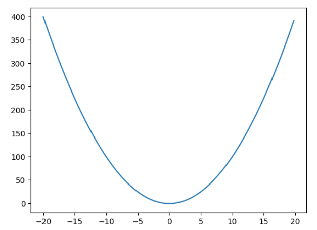
, which gives the solution as x = 0. But what if you don’t know this and need to rely on a method which can reach the minimum of a function iteratively. That is what gradient descent does.

    Gradient descent as the name suggests is like slowly descending down the mountain that is the loss function but in an iterative manner. We always take a small step in the opposite direction of the gradient. If the gradient is positive, we take a negative step and if the gradient is negative then we take a positive step.

    So in this example suppose we have to minimise x^{2} 
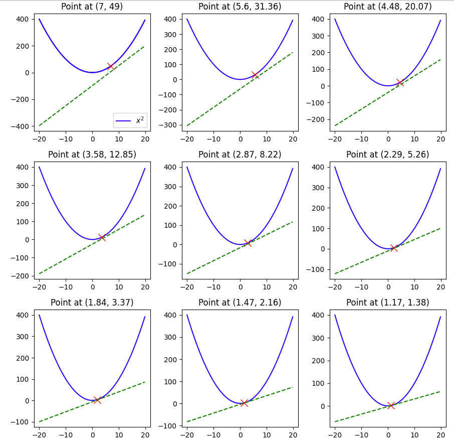
and we start off with an initial value say 7. Then we we will update the value of x as –

    x_new = x_old + (-\frac{\partial f(x)}{\partial x})*x_old*lr

    where lr is the learning rate. Tuning this value is crucial is how fast we reach the minimum, or if we overshoot the minimum and never reach it.

    Let’s take an example in python –

    import matplotlib.pyplot as plt
    import matplotlib.animation as animation
    import numpy as np

    def f(x):
    return x**2

    def derivative(x):
    return 2*x

    y = [f(x) for x in np.arange(-20,20,0.2)]
    x = np.arange(-20,20,0.2)

    plt.plot(x,y)

    value = 7
    lr = 0.1
    derivatives = []
    values = []
    for i in range(9):
    values.append(value)
    derivatives.append(derivative(value))
    value = value - lr*derivative(value)

    # List of points and derivatives
    points = [(x,f(x)) for x in values]

    # Create a 9x9 subplot grid
    fig, axs = plt.subplots(3, 3, figsize=(9, 9))


    # Plot the main plot (x^2) in the top-left subplot
    axs[0, 0].plot(x, y, label='$x^2$', color='blue')
    axs[0, 0].legend()

    # Iterate over points and derivatives to create subplots
    for i, (point_x, point_y) in enumerate(points):
    # Calculate the line passing through the point with the slope from the derivatives list
    slope = derivatives[i]
    line_y = x + slope * (x - point_x)

    axs[i//3, i%3].plot(x, y, color='blue')

    # Plot the point
    axs[i//3, i%3].plot(point_x, point_y, marker='x', markersize=10, color='red', label='Point')

    # Plot the line passing through the point with the specified slope
    axs[i//3, i%3].plot(x, line_y, linestyle='--', color='green', label=f'Slope = {slope}')

    # Set titles for subplots
    axs[i//3, i%3].set_title(f'Point at ({np.round(point_x,2)}, {np.round(point_y,2)})')

    # Adjust layout for better visualization
    plt.tight_layout()

    # Show the plot
    plt.show()

    Here we see that with a learning rate of 0.1 and a starting value of 7 and in 9 steps we were able to reach 1.17, pretty close to the minimum of 0, but not quite so, if we change the lr to 0.3, let’s see what happens.

    The minimum of 0 was reached within 9 steps.

    But what happens if we make the lr 1 –

    Here you can see that the value keeps oscillating between 7 and -7, and thus having a large learning rate also can be harmful when using ML models that use gradient descent.

    Hopefully this example gave you a visual guide on how gradient descent works.

  • Custom Objective Function in XGBoost

    In the previous post, we covered how you can create a custom loss function in Catboost, but you might be using catboost, so how can you create the same if you’re using Xgboost to train your models. In this post, I’ll walk over an example using the famous Titanic dataset, where we’ll recreate the LogLoss function and compare the results with the standard implementation in the library.

    First, we have to set up the data.

    import numpy as np 
    import seaborn as sns
    import pandas as pd
    import xgboost as xgb
    from sklearn.metrics import log_loss

    data = sns.load_dataset('titanic')

    Then some data cleaning and setting up the training dataset. The goal is not to get the best model but to demonstrate the custom loss function, so not much feature engineering is being done.

    data['embarked'].fillna('S', inplace = True)

    X,y = data[[c for c in data.columns if c not in \
    ['survived', 'alive', 'deck', 'embark_town']]], \
    data['survived']

    cat_columns = ['pclass', 'sex', 'sibsp', 'parch', 'embarked', 'class',
    'who', 'adult_male', 'alone']

    X = pd.get_dummies(X, columns=cat_columns, drop_first=True)

    Let’s say there was no loss function like logloss, then how would you define the logloss as an objective function.

    LogLoss = -1/N \sum({y_{i}log(\hat{y}) + (1-y_{i})log(1-\hat{y})})

    You’ll have to calculate the first and second derivative with respect to the \hat{y}

    \Large \frac{\partial LogLoss}{\partial \hat{y}} = -\frac{y_{i}}{\hat{y}} + \frac{1-y_{i}}{1-\hat{y}}

    \Large  \frac{\partial^2LogLoss }{\partial \hat{y}^2} = \frac{y_{i}}{\hat{y}^{2}} + \frac{1-y_{i}}{(1-\hat{y})^{2}}

    Now we will write these up as Python functions and create a function that returns the gradient and hessian (second derivative) values. In the xgboost library, the first value being passed is the predictions and the second is the training matrix.

    def log_loss_derivative(y_pred, dtrain ):
    y = dtrain.get_label()
    return (-y/y_pred) + ((1-y)/(1-y_pred))

    def log_loss_second_derivative(y_pred, dtrain):
    y = dtrain.get_label()
    return (y/np.power(y_pred,2)) + ((1-y)/np.power((1-y_pred),2))

    def custom_log_loss(predt, dtrain):
    y_pred = np.clip(predt, a_max=1-1e-5, a_min=1e-5)
    grad = log_loss_derivative(y_pred= y_pred, dtrain = dtrain)
    hess = log_loss_second_derivative(y_pred= y_pred, dtrain = dtrain)
    return grad, hess

    We clip the predictions to avoid division by zero errors. Now let’s train.

    import xgboost as xgb

    dtrain =xgb.DMatrix(data=X, label=y)

    model = xgb.train({'tree_method': 'hist', 'seed': 1994},
    dtrain=dtrain,
    num_boost_round=10,
    obj=custom_log_loss)

    log_loss(y_pred=np.clip(model.predict(dtrain), a_max=1, a_min=0), y_true=y)
    >>>0.24912

    Comparison with the standard implementation.

    clf = xgb.XGBClassifier(n_estimators = 10, **{'tree_method': 'hist', 'seed': 1994})
    clf.fit(X,y)

    log_loss(y_pred=np.clip(clf.predict_proba(X)[:,1], a_max=1, a_min=0), y_true=y)

    >>>0.2861

    As we can see the metrics are very close in our implementation of the LogLoss and the standard implementation. Of course, you should use the standard implementation when it’s available, but in case you want to use a custom loss function, you now know how to do so.

  • Creating a Custom Loss Function For Machine Learning Models

    While standard Machine Learning Libraries provide a vast array of loss functions out of the box, sometimes we need to create our own custom loss function. In this blog post, I’ll go over a simple example and create a custom loss function in Catboost.

    First we will create the data for training.

    # Importing libraries
    import numpy as np
    import pandas as pd
    from sklearn.metrics import mean_squared_error
    from catboost import CatBoostRegressor, Pool
    from sklearn.datasets import fetch_california_housing

    raw_data = fetch_california_housing()

    data = pd.concat([pd.DataFrame(raw_data['data'], columns=raw_data['feature_names']),
    pd.Series(raw_data['target'], name = 'target')], axis = 1)

    features = [i for i in data.columns.tolist() if i != 'target']

    Since the objective is not to create the best model possible, we won’t be doing any feature engineering. Let’s use catboost, and create a model using standard loss functions.

    model = CatBoostRegressor(loss_function='RMSE', n_estimators=100, eval_metric='RMSE')

    cb_pool = Pool(data=data[features], label=data['target'], feature_names=features)

    model.fit(cb_pool)

    predictions = model.predict(cb_pool)

    mean_squared_error(y_true=data['target'], y_pred=predictions)

    Upon evaluating the model we find that the mean squared error is 0.15. Definitely a model which is overfitting, but that’s not a concern for this tutorial.

    But what is you don’t want to use RMSE as a loss function, and instead want to use something like this –

    loss = \frac{\sum (y - \hat{y})^{4}}{n}

    Then how do you create a loss function in catboost?

    For this, you’ll need to calculate the first derivative and the second derivative of the loss function with respect to \hat{y}.

    Using the chain rule, the first derivative is

    \frac{\partial (y-\hat{y})^4}{\partial \hat{y}} = \frac{\partial (y-\hat{y})^4}{\partial (y-\hat{y})}*\frac{\partial y - \hat{y}}{\partial \hat{y}} = 4 * (y - \hat{y})^{3}* -1 = -4(y -\hat{y})^{3}

    And similarly using the chain rule, the second derivative comes out to be 12*(y-\hat{y})^2

    The catboost template for a custom objective is as follows –

    class UserDefinedObjective(object):
        def calc_ders_range(self, approxes, targets, weights):
            """
            Computes first and second derivative of the loss function 
            with respect to the predicted value for each object.
    
            Parameters
            ----------
            approxes : indexed container of floats
                Current predictions for each object.
    
            targets : indexed container of floats
                Target values you provided with the dataset.
    
            weight : float, optional (default=None)
                Instance weight.
    
            Returns
            -------
                der1 : list-like object of float
                der2 : list-like object of float
    
            """
            pass
    

    Using this temple, we can write the custom objective –

    class CustomLossObjective(object):
    def calc_ders_range(self, approxes, targets, weights):
    assert len(approxes) == len(targets)
    if weights is not None:
    assert len(weights) == len(approxes)

    result = []
    n = len(targets) # Number of samples

    for index in range(len(targets)):
    error = targets[index] - approxes[index]
    der1 = -4 * error**3
    der2 = 12 * error**2

    if weights is not None:
    der1 *= weights[index]
    der2 *= weights[index]

    result.append((der1, der2))
    return result

    Now let’s use this custom loss in our model

    model = CatBoostRegressor(loss_function=CustomLossObjective(), n_estimators=100, eval_metric='RMSE')
    model.fit(cb_pool)

    predictions = model.predict(cb_pool)
    mean_squared_error(y_true=data['target'], y_pred=predictions)

    Using this loss, we see that the mean squared error is 0.735, this is clearly inferior to using RMSE, but as mentioned before the objective of this blog post is not to build the best model but to showcase how one can create a custom loss objective in catboost.