Author: sahaymaniceet

  • PDF ChatBot Demo with Gradio, Llama-2 and LangChain

    PDF ChatBot Demo with Gradio, Llama-2 and LangChain

    In this post, we will learn how you can create a chatbot which can read through your documents and answer any question. In addition, we will learn how to create a working demo using Gradio that you can share with your colleagues or friends.

    The google collab notebook can be found here.

  • Fine Tune Llama-2-13b on a single GPU on custom data.

    In this tutorial, we will walk through each step of fine-tuning Llama-2-13b model on a single GPU. I’ll be using a collab notebook but you can use your local machine, it just needs to have around 12 Gb of VRAM.

    The required libraries can be installed by running this in your notebook.

    !pip install -q transformers trl peft huggingface_hub datasets bitsandbytes accelerate

    First login to your huggingface account.

    from huggingface_hub import login
    login("<your token here>")

    Loading the tokenizer.

    model_id = "meta-llama/Llama-2-13b-chat-hf"
    import torch
    device = torch.device("cuda") if torch.cuda.is_available() else torch.device("cpu")
    
    from transformers import AutoTokenizer, AutoModelForCausalLM, Trainer, TrainingArguments, BitsAndBytesConfig
    
    tokenizer = AutoTokenizer.from_pretrained(model_id)
    tokenizer.pad_token = tokenizer.eos_token

    Now we will load the model in its quantised form, this reduces the memory requirements to fit the model, so it can run on a single GPU.

    bnb_config = BitsAndBytesConfig(load_in_4bit=True,
        bnb_4bit_quant_type="nf4",
        bnb_4bit_compute_dtype=torch.bfloat16,
        bnb_4bit_use_double_quant=False)

    If you’ve a bit more GPU to play around, you can load the 8-bit model. Play around with this configuration based on your hardware specifications.

    model = AutoModelForCausalLM.from_pretrained(model_id,  quantization_config=bnb_config, use_cache=False)

    Now the below lines of code prepare the model for 4 or 8-bit training, otherwise, you get an error.

    from peft import prepare_model_for_kbit_training, get_peft_model, LoraConfig, TaskType
    
    model.gradient_checkpointing_enable()
    model = prepare_model_for_kbit_training(model)

    Then you define your LoRA config, mainly there are two parameters that you play around with – rank and lora_alpha. For more details, you can read about the params here.

    peft_config = LoraConfig(
        task_type=TaskType.CAUSAL_LM, 
        inference_mode=False, 
        r=64, 
        lora_alpha=32, 
        lora_dropout=0.1,
    )
    model = get_peft_model(model, peft_config)
    

    Now the below cell is a helper function that shows how many trainable parameters are there.

    def print_trainable_parameters(model):
        """
        Prints the number of trainable parameters in the model.
        """
        trainable_params = 0
        all_param = 0
        for _, param in model.named_parameters():
            all_param += param.numel()
            if param.requires_grad:
                trainable_params += param.numel()
        print(
            f"trainable params: {trainable_params} || all params: {all_param} || trainable%: {100 * trainable_params / all_param}"
        )
    
    print_trainable_parameters(model)
    
    >>> trainable params: 52428800 || all params: 6724408320 || trainable%: 0.7796790067620403

    We can see with LoRA, there are very few parameters to train.

    To prepare your data, you can have it in any form you want, as long as it is with datasets, you can pass a formatting function while training, which can combine all text part of the data.

    Here you can change the training configurations, For LoRA you can start with a higher learning rate as the original weights are frozen, so you don’t have to worry about catastrophic forgetting. The arguments you want to play around with are per_device_train_batch_size and gradient_accumulation_steps as when you run out of memory then lower per_device_train_batch_size and increase gradient_accumulation_steps.

    max_seq_length = 512
    
    from transformers import TrainingArguments, EarlyStoppingCallback
    from trl import SFTTrainer
    output_dir = "./results"
    optim = "paged_adamw_32bit"
    training_args = TrainingArguments(
        output_dir=output_dir,
        overwrite_output_dir=True,
        optim=optim,
        learning_rate=1e-4,
        logging_steps=10,
        max_steps=300,
        warmup_ratio=0.3,
        per_device_train_batch_size=8,
        gradient_accumulation_steps=4,
        gradient_checkpointing=True,
        save_total_limit = 5,
        fp16=True
        
    )
    

    Here I’m writing an example of a formatting function. My data already had a text field which had all the text data.

    def format_function(example):
        return example['text']

    But in case you don’t have text field, you can have it so that the function returns all text as one.

    Now we define the trainer.

    from trl import SFTTrainer
    peft_trainer = SFTTrainer(
        model=model,
        train_dataset=dataset,
        peft_config=peft_config,
        max_seq_length=max_seq_length,
        tokenizer=tokenizer,
        args=training_args,
        formatting_func=format_function)
    
    peft_trainer.train()

    Once the model has been trained, you can store is locally or push it to huggingface hub.

    Hope this tutorial cleared any doubts you had around fine-tuning LLMs on a single GPU.

  • Fine Tune Llama-2-7b with a custom dataset on google collab

    Fine Tune Llama-2-7b with a custom dataset on google collab

    I’ll add the code and explanations as text here, but everything is explained in the Youtube video.

    Link to collab notebook.

  • Understanding Naive Bayes – A simple yet powerful ML Model Part 1 – Bayes Theorem

    Naive Bayes is often not given enough credit, people when learning about ML often directly start using XgBoost or Random Forest models. While these models are good and will often achieve the task, we should also know about Naive Bayes, a Bayesian ML model, which was once used in production by tech giants like Google.

    But before we deep dive into Naive Bayes, we’ve to learn about the Bayes theorem itself.

    P(A/B) = \frac{P(B/A)*P(A)}{P(B)}

    It may seem daunting, but at its core, the formula is very simple to understand, all it provides is a way to calculate the probability of A given B has already happened. It is equal to the probability of B given that A has already happened multiplied by the probability of A divided by the probability of B happening.

    You might be daunted by mathematical jargon such as posterior and priors, but if you think in these simple terms then it is a very simple formula.

    Let’s take an example, and suppose that we don’t know Bayes theorem.

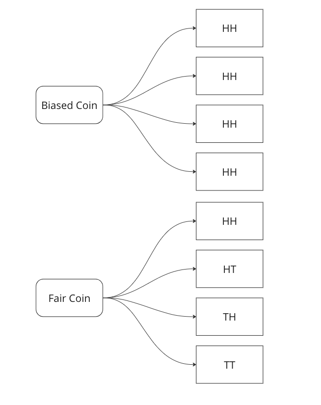
    We are told that a coin could be fair, or biased (always comes up heads). We observe two heads in a row and we have to find the probability that the coin being tossed is a fair coin.

    Graphing all outcomes of two coin tosses by both a fair and a biased coin. Now we know that two heads came in a row. So we update our sample space with this given information.

    Here we can see that we can only attribute 1 sample out of 5 to a fair coin, so P(fair coin/HH) = 1/5. In a similar way, we can say P(biased coin/HH) = 4/5 as we can attribute 4 out of 5 sample points to the biased coin.

    Let us see if we can arrive on the same answer by using the Bayes Formula.

    P(fair coin/HH) = \frac{P(HH/fair coin)*P(fair coin)}{P(HH)} = \frac{1/4*1/2}{1*1/2+1/2*1/4}=1/5

    Breaking down the calculations –

    1. P (HH/fair coin) = 1/4 – we saw above that in 1/4 cases a fair coin will give two heads
    2. P ( fair coin) = 1/2 – we know that a coin could be biased or fair, this is what is known as a prior, here it is equally likely that the coin could be biased or fair.
    3. P (HH) = 1/2*1 + 1/2*1/4 – This is where most of the confusion rises related to Bayes theorem. We have to calculate the probability of getting two heads, considering both scenarios. In the case of a biased coin, it will always gives head, so the probability is 1. There is also half a chance to select it, so we multiply it by 0.5. Similarly, we know 1/4 is the probability to get HH with a fair coin, and there is 0.5 probability to select it.

    In the next part we will see how we can use this to create a very basic classifier in Python.

  • Book Review – Inspired by Marty Cagan

    As Data Scientists, we should always try to understand the product side of things as well. A good product is useless if there is no demand for it. Inspired: How to Create Tech Products Customers Love gives us an insight into what a good product manager should do and also how should he interact or work with designers and engineers to get the best out of them.

    The book is divided into three parts: discovery, delivery, and scale. In the discovery phase, Cagan discusses the importance of understanding user needs, defining a product vision, and creating a high-fidelity prototype. In the delivery phase, he covers topics such as iterative development, team collaboration, and product launch. In the scale phase, he discusses how to grow a product and create a sustainable business.

    Like all books related to management or ways of working, it often repeats itself but there are a few major takeaways which I really liked. The emphasis on speaking with the users and the creation of a high-fidelity prototype and the reasoning behind it was key learning points for me. The book also covers the importance of testing and having good test frameworks, which although standard practice within software engineering, is often lacking with Data Scientists.

    There are a few cons as well, like it’s repetitive, a lot, like we get it, there should be a product vision, having an entire section on it felt unnecessary. It also emphasises that everyone who is working on a product should share the same working space. In modern work dynamics, this idea seems a bit dated.

    My final verdict will be that it’s worth a read due to its concepts on product prototyping and iteration.

    Rating: 3.5 out of 5.
  • Large Language Model (LLM) Evaluation Metrics – BLEU and ROUGE

    How are language models evaluated? In traditional machine learning, we have metrics like accuracy, f1-score, precision, recall etc. But how can you calculate objectively how the model performed, when the label is I like to drink coffee over tea and the model’s output is I prefer coffee to tea. As humans, we can clearly see that these two have the same meaning, but how can a machine make the same evaluation?

    Well, there are two approaches –

    1. BLEU – Bilingual Evaluation Understudy is a metric used to evaluate the quality of machine-generated translations against one or more reference translations. It measures the similarity between the machine-generated translation and the reference translations based on the n-grams (contiguous sequences of n words) present in both. BLEU score ranges from 0 to 1, with a higher score indicating a better match between the generated translation and the references. A score of 1 means a perfect match, while a score of 0 means no overlap between the generated and reference translations.
    2. ROUGE – Recall-Oriented Understudy for Gisting Evaluation) is a widely used evaluation metric for assessing the quality of automatic summaries generated by text summarization systems. It measures the similarity between the generated summary and one or more reference summaries. ROUGE calculates the precision and recall scores by comparing the n-gram units (such as words or sequences of words) in the generated summary with those in the reference summaries. It focuses on the recall score, which measures how much of the important information from the reference summaries is captured by the generated summary.

    Let us take an example and calculate both the metrics. Suppose the label is "The cat sat on the mat." and the model’s output is "The dog slept on the couch."

    Here is the python code to calculate ROUGE score –

    from collections import Counter
    import re
    
    
    def calculate_ROUGE(generated_summary, reference_summary, n):
        # Tokenize the generated summary and reference summary into n-grams
        generated_ngrams = generate_ngrams(generated_summary, n)
        reference_ngrams = generate_ngrams(reference_summary, n)
    
        # Calculate the recall score
        matching_ngrams = len(set(generated_ngrams) & set(reference_ngrams))
        recall_score = matching_ngrams / len(reference_ngrams)
    
        return recall_score
    
    
    def generate_ngrams(text, n):
        # Preprocess text by removing punctuation and converting to lowercase
        text = re.sub(r'[^\w\s]', '', text.lower())
    
        # Generate n-grams from the preprocessed text
        words = text.split()
        ngrams = [tuple(words[i:i+n]) for i in range(len(words) - n + 1)]
    
        return ngrams
    
    
    # Example usage
    generated_summary = "The dog slept on the couch."
    reference_summary = "The cat sat on the mat."
    n = 2  # bigram
    
    rouge_score = calculate_ROUGE(generated_summary, reference_summary, n)
    print(f"ROUGE-{n} score: {rouge_score}")
    >> ROUGE-2 score: 0.2
    

    If we use n = 2, which means bigrams, then the ROUGE-2 score is 0.2 .

    Similarly, lets calculate the BLEU score –

    from collections import Counter
    import nltk.translate.bleu_score as bleu
    
    
    def calculate_BLEU(generated_summary, reference_summary, n):
        # Tokenize the generated summary and reference summary
        generated_tokens = generated_summary.split()
        reference_tokens = reference_summary.split()
    
        # Calculate the BLEU score
        weights = [1.0 / n] * n  # Weights for n-gram precision calculation
        bleu_score = bleu.sentence_bleu([reference_tokens], generated_tokens, weights=weights)
    
        return bleu_score
    
    
    # Example usage
    generated_summary = "The dog slept on the couch."
    reference_summary = "The cat sat on the mat."
    n = 2  # Bigram
    
    bleu_score = calculate_BLEU(generated_summary, reference_summary, n)
    print(f"BLEU-{n} score: {bleu_score}")
    >> BLEU-2 score: 0.316227766016838
    

    So, we get two different scores from these two different approaches.

    The evaluation metric you will chose to fine tune your LLM models will depend on the task at hand, but usually BLEU is used for machine translations and ROUGE is used for summarisation tasks.

  • Machine Learning In Production – Skew and Drift

    In this post we will go over a very important concept when it comes to Machine Learning models, especially when you deploy them in production.

    Drift: Drift, or concept drift, refers to the phenomenon where the statistical properties of the target variable or the input features change over time. In other words, the relationship between the input variables and the target variable is no longer stable. This can occur due to various reasons such as changes in the underlying data-generating process, changes in user behaviour, or changes in the environment. Concept drift can have a significant impact on the performance of machine learning models because they are trained on historical data that may no longer be representative of the current state. Models may need to be continuously monitored and updated to adapt to concept drift, or specialized techniques for handling concept drift, such as online learning or ensemble methods, can be employed.

    To measure this type of skew, you can use various statistical measures –

    1. Feature Comparison: Calculate summary statistics (such as mean, median and variance) for each feature in the training dataset and the production dataset. Compare these statistics to identify any significant differences. You can use measures like the Kolmogorov-Smirnov test or the Jensen-Shannon divergence to quantify the skew between the distributions.
    2. Domain Expertise: Consult with domain experts or stakeholders who are familiar with the data and understand the expected distribution of features. They can provide insights into potential skewness or changes in feature distributions that might be critical to consider.
    3. Monitoring and Drift Detection: Implement a monitoring system to track the distribution of features in the production environment continuously. There are various drift detection algorithms available, such as the Drift-Detection Method (DDM) or the Page-Hinkley Test. These methods analyze the incoming data over time and detect significant changes or shifts in the feature distributions.

    By combining these techniques, you can gain insights into the skewness between the training and production feature distributions. Detecting and addressing such skewness is crucial for maintaining the performance and reliability of machine learning models in real-world scenarios.

  • Time Series Forecasting with Python – Part IV – Stationarity and Augmented Dicky Fuller Test

    In Part III, we saw trends and seasonality in time series data and how can we decompose it using statsmodel.

    In this part we will learn about stationarity in time series data and how can we test it using Augmented Dicky Fuller Test.

    Stationarity is a fundamental concept in time series analysis. It refers to the statistical properties of a time series remaining constant over time. In a stationary time series, the mean, variance, and autocovariance structure do not change with time.

    There are three main components of stationarity:

    1. Constant Mean: The mean of the time series should remain constant over time. This means that the average value of the series does not show any trend or systematic patterns as time progresses.
    2. Constant Variance: The variance (or standard deviation) of the series should remain constant over time. It implies that the spread or dispersion of the data points around the mean should not change as time progresses.
    3. Constant Autocovariance: The autocovariance between any two points in the time series should only depend on the time lag between them and not on the specific time at which they are observed. Autocovariance measures the linear relationship between a data point and its lagged values. In a stationary series, the autocovariance structure remains constant over time.

    Why is stationarity important in time series analysis? Stationarity is a crucial assumption for many time series models and statistical tests. If a time series violates the stationarity assumption, it can lead to unreliable and misleading results. For example, non-stationary series may exhibit trends, seasonality, or other time-dependent patterns that can distort statistical inference, prediction, and forecasting.

    To analyze non-stationary time series, researchers often use techniques like differencing to transform the series into a stationary form. Differencing involves computing the differences between consecutive observations to remove trends or other time-dependent patterns. Other methods, such as detrending or deseasonalizing, can also be employed depending on the specific characteristics of the series.

    It is important to note that while stationarity is desirable for many time series models, there are cases where non-stationary time series analysis is appropriate, such as when studying trending or seasonal data. However, in such cases, specialized models and techniques designed for non-stationary series need to be employed.

    Testing for Stationarity

    In Python, you can use various statistical tests to check for stationarity in a time series. One commonly used test is the Augmented Dickey-Fuller (ADF) test. The statsmodels library provides an implementation of the ADF test, which can be used to assess the stationarity of a time series.

    Here’s an example of how to perform the ADF test in Python:

    import pandas as pd
    from statsmodels.tsa.stattools import adfuller
    
    # Create a time series dataset
    data = [1, 2, 3, 4, 5, 6, 7, 8, 9, 10]
    
    # Perform the ADF test
    result = adfuller(data)
    
    # Extract the test statistic and p-value
    test_statistic = result[0]
    p_value = result[1]
    
    # Print the results
    print("ADF Test Statistic:", test_statistic)
    print("p-value:", p_value)
    

    The values come out to be

    ADF Test Statistic: 0.0
    p-value: 0.958532086060056

    The ADF test statistic measures the strength of the evidence against the null hypothesis of non-stationarity. A more negative (i.e., lower) test statistic indicates stronger evidence in favor of stationarity. The p-value represents the probability of observing the given test statistic if the null hypothesis of non-stationarity were true. A small p-value (typically less than 0.05) suggests rejecting the null hypothesis and concluding that the series is stationary. In this example we can clearly see that the null hypothesis was not rejected, meaning that the time series is not stationary.

    In the next part we will cover how we can convert non-stationary time series data to stationary time series.

  • Leave one out encoding – Encode your categorical variables to the target

    In case you want to use ML models on categorical variables, you’ve to encode them. The most common approach is one hot encoding. But what if you’ve too many categories and categorical variables, in this case, if you one hot encode, then you will end up with a very sparse matrix.

    Well there are ways you can tackle this, and I’ll be talking about one such way – Leave One Out Encoding.

    Leave-One-Out (LOO) is a cross-validation technique that involves splitting the data into training and test sets, where the test set contains a single sample, and the training set contains the remaining samples. LOO is performed for each sample in the dataset, and the model is trained and evaluated multiple times. In each split, you take the mean of the target for the category being encoded in train and add it to the test.

    Pros:

    1. Utilizes all available data: LOO ensures that each sample in the dataset is used as both a training and test instance. This maximizes the utilization of the available data and provides a more accurate estimate of model performance.
    2. Low bias: Since each training set contains all but one sample, the model is trained on almost the entire dataset. This reduces the bias introduced by other cross-validation techniques that use smaller training sets.
    3. Suitable for small datasets: LOO is particularly useful for small datasets where splitting the data into multiple folds might result in inadequate training data for model fitting.
    4. Unbiased estimator: LOO estimates tend to have lower bias compared to other cross-validation techniques, as the model is evaluated on independent samples.

    Cons:

    1. High computational cost: LOO requires training and evaluating the model as many times as there are samples in the dataset, making it computationally expensive, especially for large datasets.
    2. Variance and instability: LOO estimates can have high variance due to the high dependence between the training sets. Small changes in the data can lead to significant changes in the estimated performance. Thus, LOO estimates can be less stable than estimates obtained from other cross-validation methods.
    3. Overfitting risk: LOO can be prone to overfitting, as the model is trained on almost the entire dataset. This can result in overly optimistic performance estimates if the model is too complex or the dataset is noisy.
    4. Imbalanced class issues: If the dataset is imbalanced, LOO can lead to biased estimates, as each training set will typically contain a majority of samples from the majority class.

    Let’s walk through an examples.

    import pandas as pd
    import numpy as np
    from sklearn.model_selection import LeaveOneOut
    
    # Example data
    data = pd.DataFrame({
        'category': ['A', 'A', 'B', 'B', 'B', 'C', 'C', 'C'],
        'target': [1, 2, 3, 4, 5, 6, 7, 8]
    })
    
    # Create new column for leave-one-out encoded feature
    data['category_loo_encoded'] = np.nan
    

    Here we create a dummy data with a categorical variable and a numerical target.

    # Leave-One-Out Encoding
    loo = LeaveOneOut()
    
    for train_index, test_index in loo.split(data):
        X_train, X_test = data.iloc[train_index], data.iloc[test_index]
        
        # Calculate mean excluding the current row
        mean_target = X_train.loc[X_train['category'] == X_test['category'].values[0], 'target'].mean()
        
        # Assign leave-one-out encoded value
        data.loc[test_index, 'category_loo_encoded'] = mean_target
    
    # Display the result
    print(data)
    
    categorytargetcategory_loo_encoded
    A12
    A21
    B34.5
    B44
    B53.5
    C67.5
    C77
    C86.5

    There are also libraries that you can use which can help you with this. You can use category encoders. The advantage is that you can use parameters like sigma which adds noise and reduces overfitting.

    Here is the Python snippet on the same data.

    import category_encoders as ce
    # Create an instance of LeaveOneOutEncoder
    encoder = ce.LeaveOneOutEncoder(cols=['category'])
    
    # Perform leave-one-out encoding
    data_encoded = encoder.fit_transform(data['category'], data['target'])
    
    # Merge the encoded data with the original dataframe
    data = data.merge(data_encoded, how = 'left', left_index=True, right_index=True)
    
    # Display the result
    print(data)
    

    Here you can see we get the same result if we use category encoders as well.

    Thanks for reading and let me know in the comments in case you’ve any questions regarding Leave One Out Encoding.

  • Time Series Forecasting with Python Part 3 – Identifying Trends in Data

    While doing time series forecasting it is very important to analyse if your data has some trends, seasonality or periodicity in it. To identify if a time series has seasonality there are several techniques you can use.

    We will be using the following dummy data to see how we can test for seasonal trends in our data.

    sales = np.array([100, 120, 130, 150, 110, 130, 140, 160, 120, 140, 150, 170])
    
    quarters = ['Q1 2018', 'Q2 2018', 'Q3 2018', 'Q4 2018',
                'Q1 2019', 'Q2 2019', 'Q3 2019', 'Q4 2019',
                'Q1 2020', 'Q2 2020', 'Q3 2020', 'Q4 2020']
    
    1. Visual inspection – Just by looking at the plot of the time series, you can identify that there are visible patterns in it.

    In the image above you can clearly see that the sales grow from Q1 to Q3 and then decline in Q4 year on year.

    2. Autocorrelation Function (ACF) – Autocorrelation refers to the correlation of a series with itself at different time lags. In other words, it quantifies the similarity or relationship between a data point and its preceding or lagged observations. The ACF helps identify any repeating patterns or dependencies within the time series data.

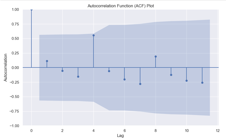
    In the ACF plot, if we see spikes at regular lag intervals, it indicates seasonality. We can take the help of plot_acf from the statsmodels package.

    import numpy as np
    import pandas as pd
    import matplotlib.pyplot as plt
    import statsmodels.api as sm
    from statsmodels.graphics.tsaplots import plot_acf
    
    # Generate ACF plot
    fig, ax = plt.subplots(figsize=(10, 6))
    plot_acf(sales, lags=11, ax=ax)  # Set lags to the number of quarters (12) minus 1
    
    plt.title('Autocorrelation Function (ACF) Plot')
    plt.xlabel('Lag')
    plt.ylabel('Autocorrelation')
    plt.show()
    

    Here we can clearly see a spike at 4, indicating what we already know that there is a seasonality present within the time series data.

    3. Decomposition –

    Decomposition is a technique used to break down a time series into its individual components: trend, seasonality, and residual (also known as error or noise). The decomposition process allows us to isolate and analyze these components separately, providing insights into the underlying patterns and variations within the time series data.

    There are two commonly used types of decomposition:

    1. Additive
    2. Multiplicative.
    1. Additive Decomposition: In additive decomposition, the time series is assumed to be the sum of its components. It is expressed as:Y(t) = Trend(t) + Seasonality(t) + Residual(t)
      The additive decomposition assumes that the magnitude of the seasonal fluctuations remains constant throughout the time series.
    2. Multiplicative Decomposition: In multiplicative decomposition, the time series is assumed to be the product of its components. It is expressed as:Y(t) = Trend(t) * Seasonality(t) * Residual(t)
      Multiplicative decomposition assumes that the seasonal fluctuations grow or shrink proportionally with the trend.

    Again we will be using the statsmodels package to perform seasonal decomposition.

    from statsmodels.tsa.seasonal import seasonal_decompose
    
    # Create a pandas Series with a quarterly frequency
    index = pd.date_range(start='2018-01-01', periods=len(sales), freq='Q')
    series = pd.Series(sales, index=index)
    
    # Perform seasonal decomposition
    decomposition = seasonal_decompose(series, model='additive')
    
    # Extract the components
    trend = decomposition.trend
    seasonality = decomposition.seasonal
    residuals = decomposition.resid
    
    # Plot the components
    plt.figure(figsize=(10, 8))
    plt.subplot(411)
    plt.plot(series, label='Original')
    plt.legend(loc='best')
    plt.subplot(412)
    plt.plot(trend, label='Trend')
    plt.legend(loc='best')
    plt.subplot(413)
    plt.plot(seasonality, label='Seasonality')
    plt.legend(loc='best')
    plt.subplot(414)
    plt.plot(residuals, label='Residuals')
    plt.legend(loc='best')
    plt.tight_layout()
    plt.show()
    

    In this dummy example, we can clearly see via this decomposition that there is an upwards trend in the data along with a quarterly seasonality.

    There are a couple more tests left to explore, but we will pick those up in the next part where we will continue to explore this seasonality and trends in time series data.