Mini book review – I just read invisible women by caroline Perez. This book is a must-read by anyone who is working with data. The book highlights key issues in everyday life that women deal with. Even small things such as the temperature of AC in office buildings are often set according to male norms. As data scientists, this book highlights key points that we should be aware of, like gender bias in our data and be cognizant that the tools we are building should have inclusivity at their core.
In case you want are also interested in reading the book, you can purchase it on Amazon by clicking here.
The title might be a bit of a clickbait, but MCC (Matthews Correlation Coefficient) is a critical ML metric that every Data Scientist must know.
Metrics like the F1 score focus on only one class and its performance, but if you want a balanced model then you should be optimising your model on MCC score rather than on Accuracy or F1-score.
If we calculate the F1-score then it is ~0.77, but the MCC score is ~0.19, meaning that even though the model is very good at classifying the positive class, it is not very good at the negative class.
As you can see the weights by default is uniform and the n_neighbours is by default 5. Large values of k smooth things, but a very small value of k will be unreliable and could be affected by outliers.
You can pick the optimal value of the k by tuning the hyperparameter using GridSearchCV.
Then there is the value of p, which is by 2, meaning that it uses the euclidean distance, you can set it to 1 to use Manhattan distance. This is the distance it uses to chose the nearest points for classification.
Let’s code this in python-
from sklearn.neighbors import KNeighborsClassifier
from sklearn.datasets import load_iris
from sklearn.model_selection import GridSearchCV

X, y = load_iris()['data'], load_iris()['target']

#defining the search grid
param_grid = {'n_neighbors': np.arange(3,10,1),
             'p': [1,2,3]}

grid_search = GridSearchCV(estimator=KNeighborsClassifier(), param_grid=param_grid, scoring='accuracy', cv = 3)

grid_search.fit(X,y)

print(grid_search.best_params_)
>>> {'n_neighbors': 4, 'p': 2}
print(grid_search.best_score_)
>>>0.9866666666666667
Hope this post cleared how you can use KNN in your machine learning problems, and if you want me to write about any ML topic, just drop a comment below.
NOTE – The article is under progress, I’ll be uploading the Youtube and linking the Kaggle notebook soon.
Most often the data you get in the real world for classification tasks is imbalanced. You always end up dealing with the imbalance on your own before passing it through models, but what if there was a python package, built on top of scikit-learn that could do the heavy lifting for you, that’s exactly what imbalanced-learn (imblearn) is.
I was inspired to use this package due this Kaggle Competition. I’ve linked the notebook in this post so you can refer it. But I’ll highly encourage you to watch the Youtube video below where I go over how I leverage imblearn with XgBoost to get a very good and balanced model as a baseline with very little effort.
There are many ways imblearn which you can leverage to balance your data.
The first is Synthetic Minority Oversampling Technique (SMOTE)
To use this, all you have to do is to invoke the following code below –
from imblearn.over_sampling import SMOTE, ADASYN
X_smote, y_smote = SMOTE().fit_resample(X, y)
After this your minortity class will up-sampled. There are also variations of SMOTE which you can use to balance your data using the library.
Similarly you can call X_adasyn, adasyn = ADASYN().fit_resample(X,y) to oversample your data.
There is also another function which will balance your data, but do know that this will take a lot of time to execute, and that is SMOTEENN (Over-sampling using SMOTE and cleaning using ENN).
To call this you again have to use these two lines of code and let imblearn do the heavy lifting for you.
from imblearn.combine import SMOTEENN
X_balanced, y_balanced = SMOTEENN().fit_resample(X,y)
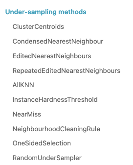
You can also use any one of the following methods to undersample your data, note that undersampling using k-nearest neighbour methods will take some time.
Again all you have to do is use <undersampling method>.fit_resample(X,y)
Once your data is ready, you can tune your model. The best thing about the competition was that the features were generated through some sort of PCA transformation, so we could easily use techniques like SMOTE, ADASYN to train the models. I did not use SMOTEENN as the notebook on Kaggle started to time out.
Here is the link to the starter notebook, you can play around with it and try other sampling methods in imblearn.
Hopefully, this post gave you insights on leveraging imblearn in your imbalanced classification problems.
This metric is usually used in multiclass classification problems. Each multiclass model gives a probability score for all the classes it is being trained on, but often you take the highest one, by using np.argmax but what if you took the top n classes and gave credit to the model if it got right in one of the n predictions. That is what is top n accuracy, it gives the model more chances to be right.
Lets take an example.
Suppose you built a model that predicts 3 classes and you want to find the top 2 accuracy of your model. Then you would pass the prediction array to the model and the true values and if the correct prediction is in the top 2 then you give it credit for being right.
import numpy as np
from sklearn.metrics import top_k_accuracy_score
y_true = [0,1,1,2,2]
y_pred = [[0.25, 0.2,0.3], #Here 0 is in the top 2
          [0.3, 0.35, 0.5], #Here 1 is in the top 2
          [0.2,0.4, 0.45], #Here 1 is in the top 2
          [0.5, 0.1, 0.2], #Here 2 is in the top 2
          [0.1, 0.4, 0.2]] #Here 2 is in the top 2
top_k_accuracy_score(y_true, y_pred, k=2)
It is 1.0, because the correct class was always in our top 2 prediction, actually, if you notice then it was always the second prediction of our model, so if we take regular accuracy or set the value k = 1 in top_k_accuracy_score(y_true, y_pred, k=2), the answer is 0.
Hopefully, this explains what top N accuracy is, and if you want me to cover any ML topic, write in the comments below. Thanks for reading.
Here are the 5 essential hyper-parameters that you should be always tuning when building any boosting model, whether you’re using XgBoost, LightGBM or even CatBoost.
n_estimators – It is not the number of trees that the boosting algorithm will grow, but as the name suggests, the number of times gradient boosting will occur, so if you are using a tree-based boosting algorithm, then if you make this number 5, then each round of boosting fits a single tree to the negative gradient of some loss function.
max_depth – The depth of each tree, pretty simple, the higher this number, the stronger each learner is in the model and the more your model can overfit. So pretty important to tune.
learning_rate – Again a very important param, the higher it is the faster your algorithm will converge to the local minima, but too high and it might overshoot the minima, too low and it might never reach the minima.
subsample – Sample of the training data to be used in each boosting round, if you use 0.5, then xgboost will randomly sample half your training data in each boosting iteration before growing the tree. Important if you want to control overfitting.
colsample_bytree – Fraction of columns to use when growing a tree, again if set to 0.5, xgboost will randomly sample half of your features to grow the tree in each boosting round. Again very important to control overfitting.
In another post I’ll be going over another 5 essential hyper-parameters that you should be tuning.
I often find people who are just starting out using pandas struggling to grasp when they should be using axis=0 and axis=1. While I go into a lot more detail with examples in the Youtube video above, you should keep this in mind.
When you use axis=0, pandas only looks at the value being passed, but when you use axis=1, by default it assumes a pandas Series being passed, so it looks for the index. So when you write a function which references multiple columns and use apply, use axis=1 and remember that it considers each row as a pandas Series, with the column names in the index.
Suppose you want to calculate aggregated count features and add them to your data frame as a feature. What you would typically do is, create a grouped data frame and then do a join. What if you can do all that in just one single line of code. Here you can use the transform functionality in pandas.
import numpy as np
import pandas as pd
import seaborn as sns
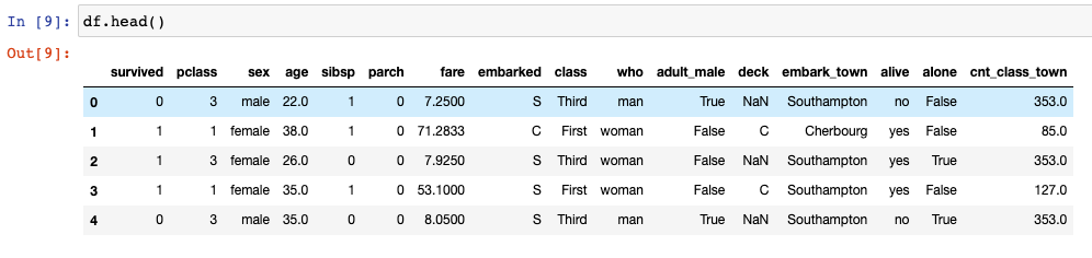
df = sns.load_dataset('titanic')
df.head()
Using df['cnt_class_town'] = df.groupby(['class', 'embark_town']).transform('size') we can directly get our desired feature in the data frame.
Again, if you want to create any sort of binned features based on the quantiles, usually first you would create a function and then use pandas apply to add that bucket to your data. Here again, you can directly use qcut functionality from pandas, pandas.qcut(x, q, labels=None, retbins=False, precision=3, duplicates='raise') to create the buckets in just one line of code.
Let’s take an example where we want to bin the age column into 4 categories, we can do so by running this one line of code –
We know that calculating the correlation between numerical variables is very easy, all you have to do is call df.corr().
But how do you calculate the correlation between categorical variables?
If you have two categorical variables then the strength of the relationship can be found by using Chi-Squared Test for independence.
The Chi-square test finds the probability of a Null hypothesis (H0).
Assumption(H0): The two columns are not correlated. H1: The two columns are correlated. Result of Chi-Sq Test: The Probability of H0 being True
We will be using the titanic dataset to calculate the chi-squared test for independence on a couple of categorical variables.
import numpy as np
import pandas as pd
import seaborn as sns
from matplotlib import pyplot as plt
df = sns.load_dataset('titanic')
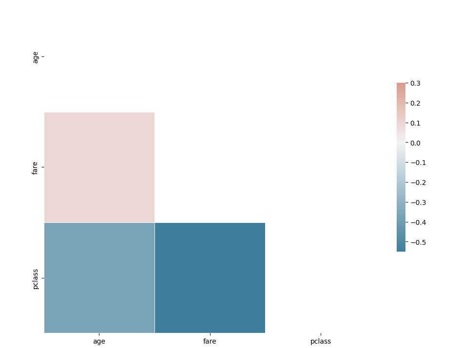
corr = df[['age', 'fare', 'pclass']].corr()
# Generate a mask for the upper triangle
mask = np.triu(np.ones_like(corr, dtype=bool))
# Set up the matplotlib figure
f, ax = plt.subplots(figsize=(11, 9))
# Generate a custom diverging colormap
cmap = sns.diverging_palette(230, 20, as_cmap=True)
# Draw the heatmap with the mask and correct aspect ratio
sns.heatmap(corr, mask=mask, cmap=cmap, vmax=.3, center=0,
square=True, linewidths=.5, cbar_kws={"shrink": .5})
Pretty easy to calculate the correlation among numerical variables.
Lets first calculate first whether the class of the passenger and whether or not they survive have a correlation.
# importing the required function
from scipy.stats import chi2_contingency
cross_tab=pd.crosstab(index=df['class'],columns=df['survived'])
print(cross_tab)
chi_sq_result = chi2_contingency(cross_tab,)
p, x = chi_sq_result[1], "reject" if chi_sq_result[1] < 0.05 else "accept"

print(f"The p-value is {chi_sq_result[1]} and hence we {x} the null Hpothesis with {chi_sq_result[2]} degrees of freedom")
The p-value is 4.549251711298793e-23 and hence we reject the null Hpothesis with 2 degrees of freedom
Similarly, we can calculate whether two categorical variables are correlated amongst other variables as well.
Hopefully, this clears up how you can calculate whether two categorical variables are correlated or not in python. In case you have any questions please feel free to ask them in the comments.
Well, the Tata Steel Chess Tournament is going on in the Netherlands, where the best Chess Players in the world, including Magnus Carlsen, are playing. They have insane chess ratings like Ding and Carlsen are rated 2800+ while the lowest rated player is 2681. Now that is some tough competition. With my measly rating of around 1200, I would not stand a chance. But the question remains, how do you come up with these ratings?
This question must have also perplexed Arpad Elo, the inventor of the Elo rating system. It tries to measure the relative skill of players in zero-sum games such as Chess. A zero-sum game is just a fancy word for saying a game where one side loses and the other side wins, or it is a draw, it cannot happen that both sides walk away with an advantageous result.
How to Calculate it?
Support player A has a rating of RA and player B has a rating of RB. Then we calculate the expected probability of a win for each of the players using the formula –
After the match player A scores SA points then we will update his rating according to the formula –
where the k-factor determines how the rating reacts to new results. If the value is set too high the ratings will jump around too much and if set too low it will take a long time to recognize greatness.
Let’s take an example. If Magnus plays against Fabi, then
#Function to calculate expected points

def expected_points(x,y):
    return 1/(1+10**((y-x)/400))

#Live ratings
r_magnus = 2850
r_fabi = 2768

#Expected points
e_magnus = expected_points(r_magnus, r_fabi)
e_fabi = expected_points(r_fabi, r_magnus)
#e_magnus = 0.615864104253756
#e_fabi = 0.384135895746244)
# If we assume that fabi wins, and a k-factor of 16, then

def new_rating(rating, k, points, expected_points):
    return rating + k*(points - expected_points)

magnus_new_rating = new_rating(r_magnus, 16, 0, e_magnus)
fabi_new_rating = new_rating(r_fabi, 16, 1, e_fabi)
Once you do the calculation, you will see that Magnus’s rating is 2840 and Fabi’s rating is now 2777.
Had Fabi lost, his rating would not go down as drastically as Magnus’s did when he lost, for example, if Fabi lost in this example, his rating will be 2761.85, so he lost lesser points when losing to a higher-rated opponent, but gains a lot if he manages to beat one. Spoiler alert – Fabi lost against Magnus in the Tata Steel Chess Tournament.
Hopefully, this post made it a bit clear how you can calculate Elo Ratings and how are they calculated for Chess Players. Fun fact, these ratings are calculated behind the scenes of almost every multi-player game to ensure that they always match you to an opponent of similar skill.


 where the k-factor determines how the rating reacts to new results. If the value is set too high the ratings will jump around too much and if set too low it will take a long time to recognize greatness.