Author: sahaymaniceet

  • Time Series Forecasting with Python – Part 2 (Moving Averages)

    In Part 1 of this series, we covered how you can use lag features and simple linear regression models to do time series forecasting, but that is very simple and you cannot capture trends using that model which is non-linear.

    So we will be discussing different types of moving averages you can calculate in python and how they are helpful.

    Simple Moving Average

    # Loading Libraries
    import numpy as np
    import pandas as pd
    import seaborn as sns
    
    sns.set_theme()
    #Using the available dowjones data in seaborn
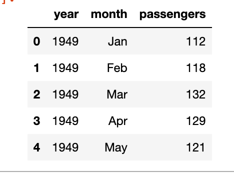
    dowjones = sns.load_dataset("dowjones")
    dowjones.head()
    

    sns.lineplot(data=dowjones, x="Date", y="Price")

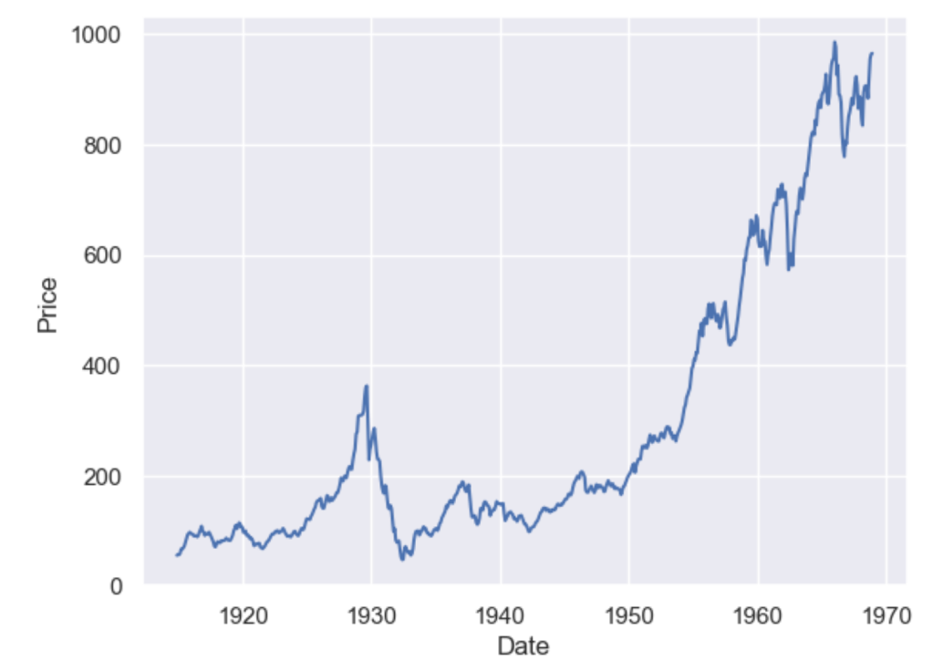
    A simple moving average (SMA) calculates the average of a selected range of values, by the number of periods in that range. The most typical moving averages are 30-day, 50-day, 100-day and 365 day moving averages. Moving averages are nice cause they can determine trends while ignoring short-term fluctuations. One can calculate the sma by simply using

    DataFrame.rolling(window, min_periods=None, center=False, win_type=None, on=None, axis=0, closed=None, step=None, method='single')

    dowjones['sma_30'] = dowjones['Price'].rolling(window=30, min_periods=1).mean()
    dowjones['sma_50'] = dowjones['Price'].rolling(window=50, min_periods=1).mean()
    dowjones['sma_100'] = dowjones['Price'].rolling(window=100, min_periods=1).mean()
    dowjones['sma_365'] = dowjones['Price'].rolling(window=365, min_periods=1).mean()
    
    sns.lineplot(x="Date", y="value", legend='auto', hue = 'variable', data = dowjones.melt('Date'))
    

    As you can see the higher the value of the window, the lesser it is affected by short-term fluctuations and it captures long-term trends in the data. Simple Moving Averages are often used by traders in the stock market for technical analysis.

    Exponential Moving Average

    Simple moving averages are nice, but they give equal weightage to each of the data points, what if you wanted an average that will give higher weight to more recent points and lesser to points in the past. In that case, what you want is to compute the exponential moving average (EMA).

    $latex EMA_{Today} = Value_{Today}(\frac{smoothing}{1+Days}) + EMA_{Yesterday}(1 – \frac{Smoothing}{1+Days})$

    To calculate this in pandas you just have to use the pandas ewm function.

    dowjones['ema_50'] = dowjones['Price'].ewm(span=50, adjust=False).mean()
    dowjones['ema_100'] = dowjones['Price'].ewm(span=100, adjust=False).mean()
    
    sns.lineplot(x="Date", y="value", legend='auto', hue = 'variable', 
                 data = dowjones[['Date', 'Price','ema_50', 'sma_50']].melt('Date'))
    

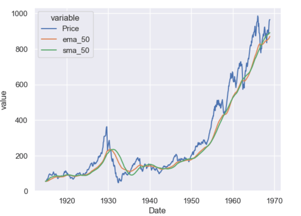
    As you can see the ema_50 follows the Price chart more closely than the sma_50 and is more sensitive to the recent data points.

    Which moving average you should use as a feature of your forecasting model is a question mostly dependent on the use case. However, you will often use some kind of moving average as a feature or to visualise long-term or short-term trends in your data.

    In Part 3 we explore trends and seasonality and how can you identify them in your data.

  • Pandas Essentials – Pivot, Pivot Table, Cast and Melt

    How to transform your data to generate insights is one of the most essential skills a Data Scientist can have. Knowing state-of-the-art models will be of no use if you cannot transform your data with ease. Pandas is a data manipulation library in python that everyone knows. It is so ubiquitous that all of us starting off in Data Science start our notebooks with import pandas as pd.

    In this post, we will go over some pandas skills that many people either don’t know, don’t use or find difficult to understand.

    As usual, you can either read the post or watch the Youtube video below.

    We will be using the flights data from seaborn as an example to go over.

    import pandas as pd
    import numpy as np
    import seaborn as sns
    flights = sns.load_dataset('flights')
    flights.head()
    

    Pivot and Pivot Table

    Now suppose that you want to create a table which had year as rows and month as columns and the passengers as values, then you will use pivot. Here is the pivot function from the official documentation of pandas – DataFrame.pivot(*index=Nonecolumns=Nonevalues=None)

    In this particular example, you’ll use year as index, month as columns and passengers in values.

    flights.pivot(index='year', columns='month', values='passengers')

    Now the most important question is why there is pivot and a pivot_table in pandas. The reason is that pivot only reshapes the data, it does not support data aggregation, for data aggregation you will have to use pivot_table.

    Now suppose I wanted to create a table which will show me for every year, what was the maximum, minimum and mean number of passengers, then there are two ways I can do it, I can either use groupby or I can use pivot_table. Here is the official documentation from pandas for pivot_table. Note: You can pass multiple aggregation functions.

    DataFrame.pivot_table(values=Noneindex=Nonecolumns=Noneaggfunc='mean'fill_value=Nonemargins=Falsedropna=Truemargins_name='All'observed=Falsesort=True)

    flights.pivot_table(values = 'passengers', index = 'year', aggfunc=[np.max, np.min, np.mean])

    Melt

    Melt is used to convert wide-form data into long-form, suppose we started with the flights data in its pivot form, that is –

    flights_wide = flights.pivot(index='year', columns='month', values='passengers')

    And we wanted to return to the flights data form, then melt can be thought of as the unpivot of pandas. To return to the original form you simply have to –

    flights_wide.melt(value_name='passengers', ignore_index=False)

    Here we don’t use an id_var as there is None, we add ignore_index as False as we want to return the index which has the year in it and we call the value_name as passengers.

    As a recap, remember that pivot makes long-form data into wide-form and melt takes wide-form data and converts it into long-form data

    So where is Cast in Pandas?

    People who have used R as a programming language often ask where is the cast functionality in pandas, the pivot_table we saw earlier is pandas’s answer to the cast functionality in Python.

  • Time Series Forecasting with Python – Part 1 (Simple Linear Regression)

    In this series of posts, I’ll be covering how to approach time series forecasting in python in detail. We will start with the basics and build on top of it. All posts will contain a practice example attached as a GitHub Gist. You can either read the post or watch the explainer Youtube video below.

    # Loading Libraries
    import numpy as np
    import pandas as pd
    import seaborn as sns
    

    We will be using a simple linear regression to predict the outcome of the number of flights in the month of May. The data is taken from seaborn datasets.

    sns.set_theme()
    flights = sns.load_dataset("flights")
    flights.head()
    

    As you can see we’ve the year, the month and the number of passengers, as a dummy example we will focus on the number of passengers in the month of May, below is the plot of year vs passengers.

    We can clearly see a pattern here and can build a simple linear regression model to predict the number of passengers in the month of May in future years. The model will be like y = slope * feature + intercept. The feature, in this case, will be the number of passengers but shifted by 1 year. Meaning the number of passengers in the year 1949 will be the feature for the year 1950 and so on.

    df = flights[flights.month == 'May'][['year', 'passengers']]
    df['lag_1'] = df['passengers'].shift(1)
    df.dropna(inplace = True)
    

    Now we have the feature, let’s build the model-

    import statsmodels.api as sm
    y = df['passengers']
    x = df['lag_1']
    model = sm.OLS(y, sm.add_constant(x))
    results = model.fit()
    b, m = results.params
    

    Looking at the results

    OLS Regression Results                            
    ==============================================================================
    Dep. Variable:             passengers   R-squared:                       0.969
    Model:                            OLS   Adj. R-squared:                  0.965
    Method:                 Least Squares   F-statistic:                     279.4
    Date:                Fri, 20 Jan 2023   Prob (F-statistic):           4.39e-08
    Time:                        17:52:21   Log-Likelihood:                -47.674
    No. Observations:                  11   AIC:                             99.35
    Df Residuals:                       9   BIC:                             100.1
    Df Model:                           1                                         
    Covariance Type:            nonrobust                                         
    ==============================================================================
                     coef    std err          t      P>|t|      [0.025      0.975]
    ------------------------------------------------------------------------------
    const         13.5750     17.394      0.780      0.455     -25.773      52.923
    lag_1          1.0723      0.064     16.716      0.000       0.927       1.217
    ==============================================================================
    Omnibus:                        2.131   Durbin-Watson:                   2.985
    Prob(Omnibus):                  0.345   Jarque-Bera (JB):                1.039
    Skew:                          -0.365   Prob(JB):                        0.595
    Kurtosis:                       1.683   Cond. No.                         767.
    ==============================================================================
    

    We can see that the p-value of the feature is significant, the intercept is not so significant, and the R-squared value is 0.97 which is very good. Of course, this is a dummy example so the values will be good.

    df['prediction'] = df['lag_1']*m + b
    sns.lineplot(x='year', y='value', hue='variable', 
                 data=pd.melt(df, ['year']))


    The notebook is uploaded as a GitHub Gist –

    Loading
    Sorry, something went wrong. Reload?
    Sorry, we cannot display this file.
    Sorry, this file is invalid so it cannot be displayed.
  • The Unicorn Project

    The Unicorn Project is the successor to The Phoenix Project, written by Gene Kim. It’s a successor and not a sequel as you don’t need to read The Phoenix Project before reading this book. It introduces new characters in the story of Parts Unlimited. The story is told from the viewpoint of Maxine, a senior lead developer.

    The story starts with Maxine being exiles to work on The Phoenix Project and there she is crippled by the way things work and she cannot even get her dev environment at the beginning and is stuck in a cycle of approvals and tickets. The book goes over familiar situations that developers and even Data Scientists or ML Engineers often come across where lack of proper infrastructure or planning of services hinder our development and delay things for weeks which can be done in hours had the design or processes been designed in a better manner.

    It’s not just a story of the issues we face in our daily work life but also about overcoming those challenges, what best practices to follow and how leaders inspire and handle pressure situations. The novel coveys some essential skills that everyone should aspire to achieve in a fun story about the struggles of working on the behemoth that is The Phoenix Project and how Maxine with her friends of rebels creates The Unicorn Project. It is a story of failure and success, of how even a senior lead developer can learn from her peers and grow despite the hurdles imposed on her by the organisation. It also showcases how it is very important to know how your customers are using the product you’re building and whether the features you are introducing will help them or not.

    The Unicorn Project is a must read for anyone working in the tech industry, whether you’re a software engineer, a DevOps or a Machine Learning Engineer, this book is for everyone.

    Rating: 4 out of 5.
  • Weight of Evidence Encoding

    So today I was participating in this Kaggle competition and the data had too many categorical variables. One way to build a model with too many categorical variables is to use a model like Catboost and let it deal with encoding categorical variables. But I wanted to ensemble my results with an Xgboost model, so I had to encode them. Using the weight of evidence encoding, I got a solution which was a top 10 solution when submitted. I have made the notebook public, you can go here and see it.

    So what is weight of evidence ?

    To put it simply –

    woe = ln(\frac{percnegatives}{percpositives}) = ln(\frac{\frac{neggroup}{totalneg}}{\frac{posgroup}{totalpos}})

    I’ve gone through an example explaining the weight of evidence in the youtube video below.

  • Linear Regression with Keras

    One often thinks that you can use deep learning for classification problems like text or image classification, or for similar tasks like segmentation, language models etc. But you can also do simple linear regression with deep learning libraries. I’ve also attached the GitHub Gist in case you want to explore the working notebook.

    In this post I’ll go over the model, it’s explanation on how can you do linear regression with keras.

    In Keras, it can be implemented using the Sequential model and the Dense layer. Here’s an example of how to implement linear regression with Keras:

    First we take a toy regression problem from scikit-learn datasets.

    from sklearn.datasets import load_diabetes
    from sklearn.model_selection import train_test_split
    
    X,y = load_diabetes(return_X_y=True)
    
    X_train, X_test, y_train, y_test = train_test_split(X,y, train_size=0.8)
    

    Now we will need to define the model using Keras. That is actually very simple, you just have to take one sequential model with a Dense layer. The activation for this layer will be linear as we’re building a linear model and the loss will be mean squared error.

    import numpy as np
    from keras.models import Sequential
    from keras.layers import Dense
    
    # define the model
    model = Sequential()
    model.add(Dense(units=1, activation='linear'))
    # compile the model
    model.compile(optimizer='sgd', loss='mean_squared_error', metrics = ['mae'])
    
    #fit the model
    model.fit(x=X_train, y=y_train, validation_data=(X_test,y_test), 
              epochs=100, batch_size=128)
    

    Thats then all that is left is to call model.predict(X_test).

    You can find the GitHub Gist below.

    Loading
    Sorry, something went wrong. Reload?
    Sorry, we cannot display this file.
    Sorry, this file is invalid so it cannot be displayed.
  • Information Gain, Gini and Decision Tree made from scratch

    In this post, we will go over the complete decision tree theory and also build a very basic decision tree using information gain from scratch.

    The below jupyter notebook as a Github Gist shows all the explanations and steps, including how to calculate Gini, Information gain and building a decision tree using the information gain you calculate.

    You can also watch the video explainer here on youtube.

    Loading
    Sorry, something went wrong. Reload?
    Sorry, we cannot display this file.
    Sorry, this file is invalid so it cannot be displayed.
  • I asked ChatGPT to write a language model

    I asked ChatGPT to write a language model. Here is the code that it returned.

    from keras.layers import Embedding, LSTM, Dense
    from keras.models import Sequential
    
    # Define the model
    model = Sequential()
    model.add(Embedding(input_dim=vocab_size, output_dim=embedding_size, input_length=max_length))
    model.add(LSTM(units=hidden_size))
    model.add(Dense(units=vocab_size, activation='softmax'))
    
    # Compile the model
    model.compile(optimizer='adam', loss='categorical_crossentropy')
    
    # Fit the model to the training data
    model.fit(x_train, y_train, batch_size=batch_size, epochs=num_epochs)


    So I decided to build a language model using it, but before I had to write a couple of lines of code myself. First the Tokenizer.

    class Tokenizer():
        def __init__(self, 
                     oov_token ='<unk>',
                     pad_token ='<pad>'):
            self.vocab = {}
            self.reverse_vocab = {}
            self.oov_token = oov_token
            self.pad_token = pad_token
            self.__add_to_dict(self.oov_token)
            self.__add_to_dict(self.pad_token)
            for i in range(10):
                self.__add_to_dict(str(i))
            for i in range(26):
                self.__add_to_dict(chr(ord('a') + i))
    
            # Add space and punctuation to the dictionary
            self.__add_to_dict('.')
            self.__add_to_dict(' ')
        
        def __add_to_dict(self, character):
            if character not in self.vocab:
                self.vocab[character] = len(self.vocab)
                self.reverse_vocab[self.vocab[character]] = character
            
        def tokenize(self, text):
            return [self.vocab[c] for c in text]
    
        def detokenize(self, text):
            return [self.reverse_vocab[c] for c in text]
        
        def get_vocabulary(self):
            return self.vocab
        
        def vocabulary_size(self):
            return len(self.vocab)
        
        def token_to_id(self,character):
            return self.vocab[character]
        
        def id_to_token(self , token):
            return self.reverse_vocab[token]
        
        def pad_seq(self,seq, max_len):
            return seq[:max_len] + [self.token_to_id(self.pad_token)]*(max_len-len(seq))
    

    Then I added the config, created a small corpus of text and prepared the training data it needs to train the model. To prepare the training data I also asked how should the corpus be created and created the corpus as it showed me.

    t = Tokenizer()
    vocab_size = t.vocabulary_size()
    embedding_size = 64
    max_length = vocab_size
    num_epochs = 50
    batch_size = 16
    
    corpus = ["this is a dog",
             "dogs live with humans", 
             "they are called what is known as pets",
             "cats are also pets",
             "there are also wolves in the jungle",
             "there are many animals in the jungle",
             "the lion is called the king of the jungle",
             "the largest animal in the jungle is the elephant",
             "we have horses also there",
             "foxes are quite quick and they are also very clever",
             "the zebra also looks like a horse but is not domesticated",
             "we go to the zoo to look at monkeys",
             "we all live together on this earth",
             'monkeys like bananas',
             'pandas eat bamboo',
             'tigers are dangerous',
             'zebras have stripes',
             'lions are the kings of the savannah',
             "it is upon humans to take care of this planet"]
    tokenized_corpus = [t.tokenize(line) for line in corpus]
    #Padding the tokenized corpus
    x_train = np.array([t.pad_seq(sentence, max_length) for sentence in tokenized_corpus])
    
    y_train = np.array([np.roll(sentence, -1) for sentence in x_train])


    Also it had a mistake in the code, which I corrected, and ran the training loop. You can find the full code here on my Github.

    I then asked ChatGPT to write the inference code for the model. Here is what it returned.

    def generate_text(seed_text, model, max_gen_length, tokenizer):
        # Tokenize the seed text
        seed_text = tokenizer.tokenize(seed_text)
        # Pad the seed text to the maximum length
        seed_text = tokenizer.pad_seq(seed_text, max_length=30)
        # Initialize an empty list to store the generated words
        generated_text = []
        # Append the seed text to the generated text
        generated_text.extend(seed_text)
        # Loop for the specified number of words to generate
        for i in range(max_gen_length):
            # Use the model to predict the next word
            next_word_probs = model.predict(np.array([seed_text]))[0]
            # Get the index of the most probable next word
            next_word_idx = np.argmax(next_word_probs)
            # Append the generated word to the generated text
            generated_text.append(next_word_idx)
            # update the seed text
            seed_text = np.delete(seed_text, 0)
            seed_text = np.append(seed_text, next_word_idx)
        # Convert the generated text from indices to words
        generated_text = [tokenizer.id_to_token(word) for word in generated_text]
        return "".join(generated_text)
    
    # Initialize the seed text
    seed_text = "The sky is"
    # Generate new text
    generated_text = generate_text(seed_text, model, max_gen_length=10, tokenizer=tokenizer)
    print(generated_text)


    Making a few changes to the code to suit our tokenizer class and model, here are a few inputs and outputs.

    Input - the sky is
    Output - the sky is<pad><pad><pad><pad><pad><pad><pad><pad><pad><pad><pad><pad><pad><pad><pad><pad><pad><pad><pad><pad><pad><pad><pad><pad><pad><pad><pad><pad><pad><pad>4444444444
    Input - "lion is the king of the jungle"
    Output - lion is the king of the jungle<pad><pad><pad><pad><pad><pad><pad><pad><pad><pad>4444444444

    Sure the output is terrible, but remember it is a very basic model architecture and we’ve not used transformers or temperature sampling to improve our language model. In my future posts, I’ll use ChatGPT to build upon these blocks to train even bigger and more complex language models.

    This shows how ChatGPT or similar large language models can enable developers in writing code or develop models in a short amount of time. It is

  • Random Projection, how it is different from PCA and where is it used

    Random projection is another dimensionality reduction algorithm like PCA, as the name suggests, the basic idea behind Random Projection is to map the original high-dimensional data onto a lower-dimensional space while preserving as much of the pairwise distances between the data points as possible. This is done by generating a random matrix of size (n x k) where n is the dimensionality of the original data and k is the desired dimensionality of the reduced data.

    If we have a matrix M of dimension mxn and another matrix R of dimension nxk whose columns are representing random directions, the random projection of M is then calculated as

    M_{p} = MR

    The idea behind random projection is similar to PCA, but in PCA we first compute the eigenvalues, here we project the vector on random directions without any complex computations.

    The random matrix used for the projection can be generated in a variety of ways. One popular method is the Johnson-Lindenstrauss lemma, which states that the pairwise distances between the points in the original space can be approximately preserved if the dimensionality of the lower-dimensional space is chosen to be logarithmic in the number of data points. Another popular method is the use of random gaussian matrix.

    The Gaussian random projection reduces the dimensionality by projecting the original input space on a randomly generated matrix where components are drawn from the following distribution N(0, \frac{1}{n_{components}}).

    Why use Random Projection in place of PCA ?

    Random Projection is often used in large-scale data analysis and machine learning applications where computational resources are limited and the dimensionality of the data is too high. In such cases, calculating PCA is often too time-consuming and computationally expensive. Additionally, Random Projection is less sensitive to the presence of noise and outliers in the data compared to PCA.

  • LeetCode #11 – Container With Most Water

    Sometimes, coding questions are also part of data science interviews, so here is the solution to LeetCode #11 – the container with the most water problem.

    The problem is very straightforward, you’re given a list with n integers, each representing the height of a tower, you’ve to find the maximum area that can be formed with these heights and the x-axis represents the index distance between the integers with a twist that since it represents a block containing water, you’ve to take the min of the two heights as the water has to contained within the towers.

    For example, if the list of given heights is h = [1,1,4,5,10,1], the maximum area that can be formed will be 8. It will be between the tower with heights 4 and 10, with an index distance of 2. So the area will be min(4,10)*2 = 8.

    Coming to the solution, the easiest solution will be to compare each combination of two tower heights, and return the maximum area that can be formed. This will have a time complexity of O(n^{2})

    def maxArea(height: List[int]) -> int:
            max_vol = 0
            for i in range(len(height)):
                for j in range(1,len(height)):
                    if j<=i:
                        continue
                    else:
                        vol = min(height[i], height[j])*(j-i)
                        max_vol = max(max_vol, vol)
            return max_vol
    

    Although the above solution will pass the sample test cases, it will eventually return Time Limit Exceeded as it is a very brute force solution, as it compares almost every possible combination. You can be a bit more clever in your approach and solve this problem in O(n) time complexity.

    The trick is using pointers, one for left and one for right, starting with the largest width and then storing the max area. Move the left pointer right if you encounter a higher tower in the left otherwise move the right pointer towards the left, and repeat till both pointers meet. In this way, you’ve traversed the list only once.

    def maxArea(height: List[int]) -> int:
            l,r = 0,len(height) - 1
            max_vol = -1
            while l < r:
                #Calculating the shorter height of the two
                shorter_height = min(height[l], height[r])
                width = r-l
                vol = shorter_height * width
                max_vol = max(vol, max_vol)
                if height[l] < height[r]:
                    l+=1
                else:
                    r-=1
            return max_vol
    

    Taking an example, if input is [1,4,5,7,4,1], then.

    Steplrwidthmin heightareamax area
    1055155
    2044145
    314341212
    41324812
    52315512
    The loop will exit after step 5 as in step 6 l = r = 3, and we get the max area as 12.