Author: sahaymaniceet

  • Essential Data Science Questions that you must know

    While the questions that you may be asked in a data science interview can vary a lot depending on the job description and the skillsets the organisation is looking for, there are a few questions that are often asked and as a candidate, you should know the answer to these.

    Here in this post I’ll try to cover 10 such questions that you should know –

    1. What is Bias-Variance Trade-off?

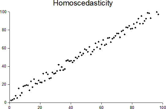
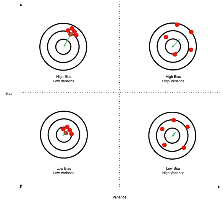
    Bias in very simple terms is the error of your ML model. Variance is the difference in the evaluation metric in the train set and the test set that your model achieves. With any machine learning model, you try to reduce both bias and variance. The bias-variance trade-off is as you reduce bias, variance usually increases. So you try to select the ML model which has the lowest bias and variance. The below diagram should explain bias and variance.

    source

    2. In multiple linear regression if you keep adding dependent variables, the coefficient of determination (R-squared value) keeps going up, how do you then measure whether the model is improving or not?

    In case of multiple linear regression, in addition to the R^{2} you also calculate the adjusted r2, R_{adj}^{2} = 1 - \frac{(1-R^{2})(n-1)}{n-p-1}, which adjusts for the number of variables in the model and penalizes models with an excessive number of variables.

    You should stop adding dependent variables when the adjusted r2 values starts to worsen

    3. How does Random Forest reduce variance?

    The main idea behind the Random Forest algorithm is to use low-bias decision trees and aggregate their results to reduce variance. Since each tree is grown from a bagged sample and also the features are bagged, meaning that each tree is grown from a different subset of features, thus the trees are not correlated and hence their combined results lead to lower variance than a single decision tree with low bias and high variance.

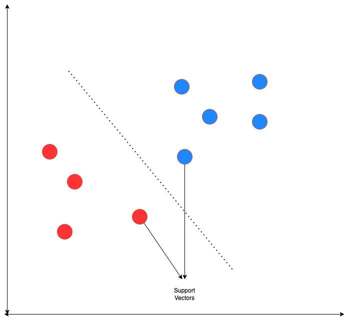
    4. What are the support vectors in support vector machine (SVM)?

    The support vectors are the data points that are used to define the decision boundary, or hyperplane, in an SVM. They are the key data points that determine the position of the decision boundary, and any change in these support vectors will result in a change in the decision boundary.

    5. What is cross-validation and how is it used to evaluate a model’s performance?

    Cross-validation involves dividing the available data into two sets: a training set and a validation set. The model is trained on the training set, and its performance is evaluated on the validation set. This process is repeated multiple times with different partitions of the data, and the performance measure is averaged across all iterations. This gives a more robust estimation of the model’s performance than a single train test split can do.

    There are different types of cross-validation methods like k-fold cross-validation, in which the data is divided into k-folds, and the model is trained on k-1 folds and tested on the remaining fold. This process is repeated k times, and the performance measure is averaged across all iterations. Another one is Leave one out Cross-validation(LOOCV), in this method we use n-1 observations for training and the last one for testing. There is also a time-series cross-validation where the model is trained till time t and tested for a time after t. The window of training time keeps expanding after each iteration, it is also called expanding window cross-validation for time series.

    I’ll be posting more Data Science questions on the blog so keep following for updates.

  • Storytelling with Data – Book Review

    Rating: 5 out of 5.

    Storytelling with Data is a must-read, not just for Data Analysts, but even for ML Engineers and Data Scientists. The book highlights the importance of how to present the analysis and draw the attention of the people consuming that information to the right places.

    I personally had this as an audiobook and had to refer to the accompanying pdf over and over again, so I recommend buying the kindle or paperback version.

    The book goes over some essential things that one should keep in mind while building a visualisation and what aspects to cover to make sure that your point is understood by the person who you’re making the visualisation for and also in the easiest way possible.

    Some of the concepts covered in the book are –

    • Choosing the right visualisation
    • Decluttering your dasboards
    • Drawing focus to the right place
    • Using colour effectively

    The book is example driven and you will find a lot of use cases which drive home the point the author is trying to make.

    In conclusion, after reading the book you will see visualisations in a different way than you did before. In case you want to buy the book you can do so here.

  • sMAPE vs MAPE vs RMSE, when to use which regression metric

    I was going through Kaggle competitions when this competition caught my eye, especially the evaluation metric for it. Now the usual metrics for forecasting or regression problems are either RMSE = \sqrt{\frac{\sum (y - \hat{y})^{2}}{N}} or MAPE = \frac{1}{N}\sum_{t=1}^{n}\frac{\left|A_{t}-F_{t}\right|}{\left|A_{t}\right|}, but sMAPE is different.

    SMAPE (Symmetric Mean Absolute Percentage Error) is a metric that is used to evaluate the accuracy of a forecast model. It is calculated as the average of the absolute percentage differences between the forecasted and actual values, with the percentage computed using the actual value as the base. Mathematically, it can be expressed as:

    sMAPE = \frac{100}{n}\sum_{t=1}^{n}\frac{\left|F_{t} - A_{t} \right|}{(\left|A_{t} \right| + \left|F_{t} \right|)/2}

    So when to use which metric ?

    • RMSE – When you want to penalize large outlier errors in your prediction model, RMSE is the metric of choice as it penalizes large errors more than smaller ones.
    • MAPE – All errors have to be treated equally, so in those cases MAPE makes sense to use
    • sMAPE – is typically used when the forecasted values and the actual values are both positive, and when the forecasts and actuals are of similar magnitudes. It is symmetric in that it treats over-forecasting and under-forecasting the same.

    It is important to note that in both MAPE and sMAPE, values of 0 are not allowed for both actual and forecast values as it would result in division by zero error.

  • Macro vs micro averages, how are they calculated ?

    In this post, I’ll go over macro and micro averages, namely precision, and recall.

    What is macro and micro averages ?

    A macro takes the measurement independently of each class and then takes the average, thus giving equal weight to each class whereas a micro will take the class imbalances into account when computing the average.

    When to use macro vs micro averages ?

    If you suspect class imbalances to be there, then micro average should be preferred to macro.

    How are they different ?

    Let’s take an example scenario from here.

    from sklearn.metrics import precision_score
    y_true = [0, 1, 2, 0, 1, 2]
    y_pred = [0, 2, 1, 0, 0, 1]
    precision_score(y_true, y_pred, average='macro')
    0.22...
    precision_score(y_true, y_pred, average='micro')
    0.33...
    

    You can see that the precision score is different for macro calculation vs micro calculation.

    Breaking down the calculation here in the confusion matrix

    A quick recap the the precision formula is for binary classification problem –

    Precision = \frac{TP}{TP+FP}


    For multi-class the micro and macro formula can be written as – Precision_{micro} = \frac{\sum TP_{i} }{\sum TP_{i}+\sum FP_{i}}


    Precision_{macro} = \frac{\sum PR_{i} }{n}


    So in the above example, the micro precision is

    Similarly the Precision for each class individually is

    P(0) = 2/3 = 0.66, P(1) = 0, P(2) = 0

    So macro precision is

    In this way the micro vs macro averages differ. Hope this article cleared your problems on macro vs micro averages in ML metrics.

  • ReLU vs Leaky ReLU, when to use what

    ReLU (Rectified Linear Unit) and Leaky ReLU are both types of activation functions used in neural networks.

    ReLU

    ReLU is defined as f(x) = max(0, x), where x is the input to the function. It sets all negative input values to zero while allowing all non-negative values to pass through unchanged. This can help speed up training and improve the performance of the model because it reduces the number of negative input values that need to be processed by the model.

    Leaky ReLU is an extension of ReLU that aims to address the problem of “dying ReLUs” in which some neurons in the network never activate because the gradient is zero for all input values less than zero. It can be defined mathematically as f(x) = max(x, kx) where k is usually a small negative slope (of 0.01 or so) for negative input values, rather than being zero as in a standard ReLU.

    In practice, LeakyReLU is being used as a generalization of ReLU. This small negative slope helps in avoiding the dying ReLU problem. Also, it helps to train a network faster as the gradients for negative input values will not be zero. A general rule of thumb when choosing between the two would be that, if the problem does not have sparse inputs and the data set is not too small, using Leaky ReLU may result in a more accurate model. Otherwise, if the problem has sparse inputs and/or the data set is small, then using ReLU is a better choice.

    It also depends on personal preferences and what the dataset is like. Sometimes leaky ReLU may work better in some cases and sometimes ReLU may be better. It’s important to try out different activation functions and see which one gives the best performance on your dataset.

  • Why Tanh is a better activation function than sigmoid ?

    You might be asked that why often in neural networks, tanh is considered to be a better activation function than sigmoid.

    Sigmoid
    Tanh

    Andrew NG also mentions in his deep learning specialization course that tanh is almost always a better activation function than sigmoid. So why is that the case?

    There are a few reasons why the hyperbolic tangent (tanh) function is often considered to be a better activation function than the sigmoid function:

    1. The output of the tanh function is centered around zero, which means that the negative inputs will be mapped to negative values and the positive inputs will be mapped to positive values. This makes the learning process of the network more stable.
    2. The tanh function has a derivative that is well-behaved, meaning that it is relatively easy to compute and the gradient is relatively stable.
    3. The sigmoid function, on the other hand, maps all inputs to values between 0 and 1. This can cause the network to become saturated, and the gradients can become very small, making the network difficult to train.
    4. Another reason is that the range of the tanh function is [-1,1], while the range of the sigmoid function is [0,1], which makes the model output values more similar to the standard normal distribution. It will be less likely to saturate and more likely to have a good gradient flow, leading to faster convergence.
    5. Another advantage is that the tanh function is differentiable at all points. In contrast, the sigmoid function has a kink at 0, which may cause issues when computing gradients during back-propagation, and other optimization methods.

    All that being said, whether to use sigmoid or tanh depends on the specific problem and context, and it’s not always the case that one is clearly better than the other.

  • When to use F2 or F0.5 score ? (F-beta score)

    Whenever we come across an imbalanced class problem, the metric to measure is often F1 score and not accuracy. A quick reminder that the F1 score is the harmonic mean of precision and recall.

    Precision is how accurate is your ML model in its predictions.

    Recall is a measure of the model’s ability to correctly identify the positive class.

    So the F1 score is a balanced measure of both recall and precision. But what if you want to prioritize reducing false positives or reducing false negatives, there comes F-beta. It’s a generalized metric, where a parameter beta is introduced to generalize the F-score.

    This enables one to choose an appropriate beta value to tune for the task at hand. If you want to minimize false positives, you want to increase the weight of precisions, so you should choose a value of beta less than 1, typically 0.5 is chosen and is called F0.5 score.

    Similarly, if you want to increase the importance of recall and reduce false negatives, you should choose a value of beta greater than 1, typically 2 is selected and is called F2 score.

    In a nutshell, you should optimize F2 score to reduce false negatives and F0.5 score to reduce false positives.

  • Oddball Data Science Interview Questions on Decision Trees

    Decision trees are the building blocks of most ML models. So often questions regarding Decision Trees are asked in data science interviews. In this post, I’ll try to cover some questions which are asked during data science interviews but often catch people by surprise.

    Are Decision Trees Parametric or non-parametric models ?

    Decision Trees are non-parametric models. Linear Regression and Logistic regression are examples of parametric models

    Why is Gini Index preferred way of growing decision trees than Entropy in Machine Learning libraries ?

    The calculation for Gini Index is computationally more effecient than that for Entropy.

    It’s because of this reason that it is the preferred way

    How are continouis variables handled as predictor variables in decision trees ?

    Continuous or numerical variables are binned and then used for splitting a node in Decision tree

    What is optimised in case the target is a continuous variable or when the task is Regression ?

    Variance reduction is used to choose the best split when the target is continuous.

    How do decision trees handle multiple classes or in other words does multi-class classification ?

    The split is done on Information gain like in case of binary classifier using Gini or Entropy. In the leaf where no further splits are possible, the class having the highest probability is the predicted class. You can even return the probability as well.

  • What is Heteroscedasticity and How do we Test for it ?

    Once your linear regression model is trained, you should always plot your residuals (y – ŷ) whether the errors are homoscedastic or heteroscedastic. What do we mean by these terms? It means that there should not be any pattern in residuals and they should be uniformly distributed, or in other words, there should not be any variance in the residuals. Homoscedasticity is one of the assumptions of linear regression, so it is often important to check for it.

    source: Wikipedia
    source: Wikipedia

    In the above figures, you can clearly see that the residuals have a clear pattern in the heteroscedastic image. In that scenario, you cannot rely on the regression analysis.

    How to test for heteroscedasticity?

    There are many ways to test for heteroscedasticity, I’ll list a. few ways here –

    1. Visual Test – Just look at the residual plot and you’ll often see whether the residuals have any variance or not, not very accurate but often works.
    2. Bartlett test
    3. Breusch Pagan test
    4. Goldfeld Quandt test
    5. Glesjer test
    6. Test based on Spearman’s rank correlation coefficient
    7. White test
    8. Ramsey test
    9. Harvey Phillips test
    10. Szroeter test
    11. Peak test (nonparametric) test

    All these tests in one way or another try to reject the null hypothesis H0 : variance is constant and the alternative hypothesis is that Ha : variance is not constant. You can go into detail about the tests here.

  • Importance of VIF in Linear Regression

    What is VIF

    Variance Inflation Factor (VIF) determines the multicollinearity amongst the independent variables (predictors). Multicollinearity is when there is a high correlation between your predictor variables, usually 0.8 or higher. This can adversely affect your regression analysis.

    How is it calculated?

    VIF of a predictor variable is calculated by regressing it against all other predictor variables. This gives the R2 value which can be plugged into this formula

    This will give the VIF value of a predictor.

    • VIF = 1, not correlated
    • VIF < 5, slightly correlated
    • VIF > 5, highly correlated

    These values are just guidelines and how high acceptable VIF values are depends on the problem statement.

    If you don’t want to use VIF and have very few predictor variables, one can plot a correlation matrix and remove the highly correlated variables.

    You might also wonder why do we calculate the p-value of predictor variables in Linear regression. Find out why here.