Category: Data Science Interview

Balanced Log Loss, Metric for imbalanced classification problems
We all know about LogLoss which is the main loss function when it comes to binary classification problems. The formula is given below –

$LogLoss = -\frac{1}{N} \sum_{i=1}^{N} \left( y_i \log(p_i) + (1 - y_i) \log(1 - p_i) \right)$
- (N) is the total number of samples.
- (y_i) is the true label of sample (i) (0 or 1).
- (p_i) is the predicted probability of sample (i) belonging to class 1.
Imbalanced Log Loss:
The imbalanced log loss accounts for class imbalance by introducing class weights. It can be defined as:

$ImbalancedLogLoss = -\frac{1}{N} \sum_{i=1}^{N} w_i \left( y_i \log(p_i) + (1 - y_i) \log(1 - p_i) \right)$
- (N) is the total number of samples.
- (y_i) is the true label of sample (i) (0 or 1).
- (p_i) is the predicted probability of sample (i) belonging to class 1.
- (w_i) is the weight assigned to sample (i) based on its class label. For example, if class 0 has fewer samples than class 1, (w_i) can be set to the ratio of class 1 samples to class 0 samples.
Here is the python code that you can call to evaluate in Catboost –
```
class BalancedLogLoss:
    def get_final_error(self, error, weight):
        return error

    def is_max_optimal(self):
        return False

    def evaluate(self, approxes, target, weight):
        y_true = target.astype(int)
        y_pred = approxes[0].astype(float)
        
        y_pred = np.clip(y_pred, 1e-15, 1 - 1e-15)
        individual_loss = -(y_true * np.log(y_pred) + (1 - y_true) * np.log(1 - y_pred))
        
        class_weights = np.where(y_true == 1, np.sum(y_true == 0) / np.sum(y_true == 1), np.sum(y_true == 1) / np.sum(y_true == 0))
        weighted_loss = individual_loss * class_weights
        
        balanced_logloss = np.mean(weighted_loss)
        
        return balanced_logloss, 0.0
```
Advantages of Imbalanced LogLoss –
1. Handles Class Imbalance: The imbalanced log loss takes into account the class distribution and assigns appropriate weights to each class. This allows the model to effectively handle imbalanced datasets, where one class may have significantly fewer samples than the other. By assigning higher weights to the minority class, the model focuses more on correctly classifying the minority class, reducing the impact of class imbalance.
2. Improves Model Performance: By incorporating class weights in the loss function, the imbalanced log loss guides the model to optimize its predictions specifically for imbalanced datasets. This can lead to improved model performance, as the model becomes more sensitive to the minority class and learns to make better predictions for both classes.
3. Flexible Weighting Strategies: The imbalanced log loss allows flexibility in assigning weights to different classes. Various weighting strategies can be used based on the characteristics of the dataset and the specific problem at hand. For example, weights can be inversely proportional to class frequencies or can be set manually based on domain knowledge. This flexibility enables the model to adapt to different levels of class imbalance and prioritize the correct classification of the minority class accordingly.
4. Evaluation Metric Consistency: When using the imbalanced log loss as both the training loss and evaluation metric, it ensures consistency in model optimization and evaluation. By optimizing the model to minimize the imbalanced log loss during training, the model’s performance is directly aligned with the evaluation metric, providing a fair assessment of the model’s effectiveness in handling class imbalance.
In conclusion, if you have an imbalanced class problem, you can try this eval metric in your models as well.

.
June 18, 2023
MCC Score – The only ML metric you need

The title might be a bit of a clickbait, but MCC (Matthews Correlation Coefficient) is a critical ML metric that every Data Scientist must know.

Metrics like the F1 score focus on only one class and its performance, but if you want a balanced model then you should be optimising your model on MCC score rather than on Accuracy or F1-score.

Let us take an example of –

y_true = [1,1,1,1,0,0,1, 0,1] y_pred = [1,1,1,1,1,1,1, 0,0]

If we calculate the F1-score then it is ~0.77, but the MCC score is ~0.19, meaning that even though the model is very good at classifying the positive class, it is not very good at the negative class.

If we look at the formula for MCC –
\[MCC = \frac{(TPxTN)-(FPxFN)}{\sqrt{(TP+FP)(TP+FN)(TN+FP)(TN+FN)}}\] https://www.hostmath.com/Math/MathJax.js?config=OK
It should be clear that MCC gives equal focus on both TP and TN, since it is a correlation coefficient, its value ranges from -1 to 1.

February 5, 2023
5 Essential Boosting Parameters You Should Be Tuning
Here are the 5 essential hyper-parameters that you should be always tuning when building any boosting model, whether you’re using XgBoost, LightGBM or even CatBoost.
1. n_estimators – It is not the number of trees that the boosting algorithm will grow, but as the name suggests, the number of times gradient boosting will occur, so if you are using a tree-based boosting algorithm, then if you make this number 5, then each round of boosting fits a single tree to the negative gradient of some loss function.
2. max_depth – The depth of each tree, pretty simple, the higher this number, the stronger each learner is in the model and the more your model can overfit. So pretty important to tune.
3. learning_rate – Again a very important param, the higher it is the faster your algorithm will converge to the local minima, but too high and it might overshoot the minima, too low and it might never reach the minima.
4. subsample – Sample of the training data to be used in each boosting round, if you use 0.5, then xgboost will randomly sample half your training data in each boosting iteration before growing the tree. Important if you want to control overfitting.
5. colsample_bytree – Fraction of columns to use when growing a tree, again if set to 0.5, xgboost will randomly sample half of your features to grow the tree in each boosting round. Again very important to control overfitting.
In another post I’ll be going over another 5 essential hyper-parameters that you should be tuning.
January 26, 2023
Pandas Essentials – Transform and Qcut
Suppose you want to calculate aggregated count features and add them to your data frame as a feature. What you would typically do is, create a grouped data frame and then do a join. What if you can do all that in just one single line of code. Here you can use the transform functionality in pandas.
```
import numpy as np
import pandas as pd
import seaborn as sns
df = sns.load_dataset('titanic')
df.head()
```
Using df['cnt_class_town'] = df.groupby(['class', 'embark_town']).transform('size') we can directly get our desired feature in the data frame.

Again, if you want to create any sort of binned features based on the quantiles, usually first you would create a function and then use pandas apply to add that bucket to your data. Here again, you can directly use qcut functionality from pandas, pandas.qcut(x, q, labels=None, retbins=False, precision=3, duplicates='raise') to create the buckets in just one line of code.

Let’s take an example where we want to bin the age column into 4 categories, we can do so by running this one line of code –

df['age_bucket'] = pd.qcut(df['age'], q = [0,0.25,0.5,0.75, 1], labels = ["A", "B", "C", "D"])

Do note that the labels have to be 1 less than your quantiles (q). The explanation as to why I have explained in the Youtube video (see above).

Hopefully, this clears up some pandas concepts and lets you write faster and neater code.
January 24, 2023
How To Calculate Correlation Among Categorical Variables?
We know that calculating the correlation between numerical variables is very easy, all you have to do is call df.corr().

But how do you calculate the correlation between categorical variables?

If you have two categorical variables then the strength of the relationship can be found by using Chi-Squared Test for independence.

The Chi-square test finds the probability of a Null hypothesis (H0).

Assumption(H0): The two columns are not correlated. H1: The two columns are correlated. Result of Chi-Sq Test: The Probability of H0 being True

We will be using the titanic dataset to calculate the chi-squared test for independence on a couple of categorical variables.
```
import numpy as np
import pandas as pd
import seaborn as sns
from matplotlib import pyplot as plt

df = sns.load_dataset('titanic')
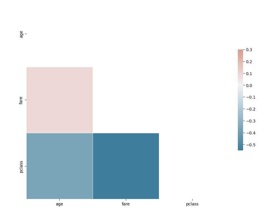
corr = df[['age', 'fare', 'pclass']].corr()

# Generate a mask for the upper triangle
mask = np.triu(np.ones_like(corr, dtype=bool))

# Set up the matplotlib figure
f, ax = plt.subplots(figsize=(11, 9))

# Generate a custom diverging colormap
cmap = sns.diverging_palette(230, 20, as_cmap=True)

# Draw the heatmap with the mask and correct aspect ratio
sns.heatmap(corr, mask=mask, cmap=cmap, vmax=.3, center=0,
            square=True, linewidths=.5, cbar_kws={"shrink": .5})
```
Pretty easy to calculate the correlation among numerical variables.

Lets first calculate first whether the class of the passenger and whether or not they survive have a correlation.
```
# importing the required function
from scipy.stats import chi2_contingency
cross_tab=pd.crosstab(index=df['class'],columns=df['survived'])
print(cross_tab)
```
```
chi_sq_result = chi2_contingency(cross_tab,)
p, x = chi_sq_result[1], "reject" if chi_sq_result[1] < 0.05 else "accept"

print(f"The p-value is {chi_sq_result[1]} and hence we {x} the null Hpothesis with {chi_sq_result[2]} degrees of freedom")
```
```
The p-value is 4.549251711298793e-23 and hence we reject the null Hpothesis with 2 degrees of freedom
```
Similarly, we can calculate whether two categorical variables are correlated amongst other variables as well.

Hopefully, this clears up how you can calculate whether two categorical variables are correlated or not in python. In case you have any questions please feel free to ask them in the comments.
January 23, 2023
Information Gain, Gini and Decision Tree made from scratch

In this post, we will go over the complete decision tree theory and also build a very basic decision tree using information gain from scratch.

The below jupyter notebook as a Github Gist shows all the explanations and steps, including how to calculate Gini, Information gain and building a decision tree using the information gain you calculate.

You can also watch the video explainer here on youtube.

Loading
Sorry, something went wrong. Reload?

Sorry, we cannot display this file.

Sorry, this file is invalid so it cannot be displayed.
Viewer requires iframe.

view raw decision_tree_from_scratch.ipynb hosted with ❤ by GitHub

January 16, 2023
Random Projection, how it is different from PCA and where is it used

Random projection is another dimensionality reduction algorithm like PCA, as the name suggests, the basic idea behind Random Projection is to map the original high-dimensional data onto a lower-dimensional space while preserving as much of the pairwise distances between the data points as possible. This is done by generating a random matrix of size (n x k) where n is the dimensionality of the original data and k is the desired dimensionality of the reduced data.

If we have a matrix M of dimension $mxn$ and another matrix R of dimension $nxk$ whose columns are representing random directions, the random projection of M is then calculated as

$M_{p} = MR$

The idea behind random projection is similar to PCA, but in PCA we first compute the eigenvalues, here we project the vector on random directions without any complex computations.

The random matrix used for the projection can be generated in a variety of ways. One popular method is the Johnson-Lindenstrauss lemma, which states that the pairwise distances between the points in the original space can be approximately preserved if the dimensionality of the lower-dimensional space is chosen to be logarithmic in the number of data points. Another popular method is the use of random gaussian matrix.

The Gaussian random projection reduces the dimensionality by projecting the original input space on a randomly generated matrix where components are drawn from the following distribution $N(0, \frac{1}{n_{components}})$ .

Why use Random Projection in place of PCA ?

Random Projection is often used in large-scale data analysis and machine learning applications where computational resources are limited and the dimensionality of the data is too high. In such cases, calculating PCA is often too time-consuming and computationally expensive. Additionally, Random Projection is less sensitive to the presence of noise and outliers in the data compared to PCA.

January 14, 2023
Essential Data Science Questions that you must know

While the questions that you may be asked in a data science interview can vary a lot depending on the job description and the skillsets the organisation is looking for, there are a few questions that are often asked and as a candidate, you should know the answer to these.

Here in this post I’ll try to cover 10 such questions that you should know –

1. What is Bias-Variance Trade-off?

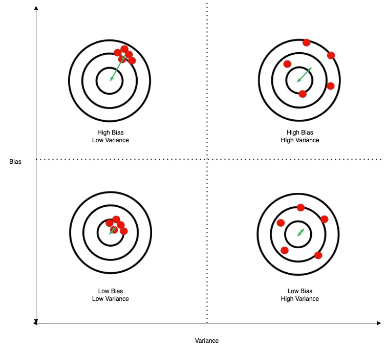
Bias in very simple terms is the error of your ML model. Variance is the difference in the evaluation metric in the train set and the test set that your model achieves. With any machine learning model, you try to reduce both bias and variance. The bias-variance trade-off is as you reduce bias, variance usually increases. So you try to select the ML model which has the lowest bias and variance. The below diagram should explain bias and variance.

source

2. In multiple linear regression if you keep adding dependent variables, the coefficient of determination (R-squared value) keeps going up, how do you then measure whether the model is improving or not?

In case of multiple linear regression, in addition to the $R^{2}$ you also calculate the adjusted r2, $R_{adj}^{2} = 1 - \frac{(1-R^{2})(n-1)}{n-p-1}$ , which adjusts for the number of variables in the model and penalizes models with an excessive number of variables.

You should stop adding dependent variables when the adjusted r2 values starts to worsen

3. How does Random Forest reduce variance?

The main idea behind the Random Forest algorithm is to use low-bias decision trees and aggregate their results to reduce variance. Since each tree is grown from a bagged sample and also the features are bagged, meaning that each tree is grown from a different subset of features, thus the trees are not correlated and hence their combined results lead to lower variance than a single decision tree with low bias and high variance.

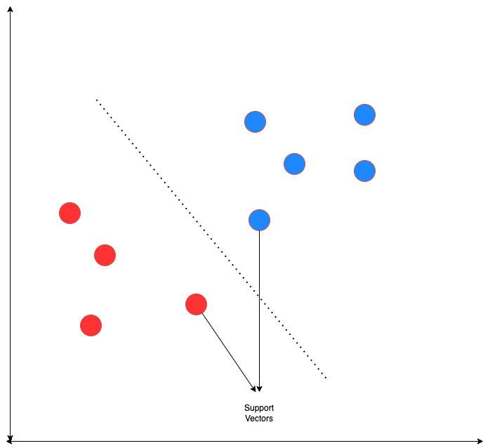
4. What are the support vectors in support vector machine (SVM)?

The support vectors are the data points that are used to define the decision boundary, or hyperplane, in an SVM. They are the key data points that determine the position of the decision boundary, and any change in these support vectors will result in a change in the decision boundary.

5. What is cross-validation and how is it used to evaluate a model’s performance?

Cross-validation involves dividing the available data into two sets: a training set and a validation set. The model is trained on the training set, and its performance is evaluated on the validation set. This process is repeated multiple times with different partitions of the data, and the performance measure is averaged across all iterations. This gives a more robust estimation of the model’s performance than a single train test split can do.

There are different types of cross-validation methods like k-fold cross-validation, in which the data is divided into k-folds, and the model is trained on k-1 folds and tested on the remaining fold. This process is repeated k times, and the performance measure is averaged across all iterations. Another one is Leave one out Cross-validation(LOOCV), in this method we use n-1 observations for training and the last one for testing. There is also a time-series cross-validation where the model is trained till time t and tested for a time after t. The window of training time keeps expanding after each iteration, it is also called expanding window cross-validation for time series.

I’ll be posting more Data Science questions on the blog so keep following for updates.

January 13, 2023