In the realm of regression analysis, one of the key metrics used to evaluate the goodness-of-fit of a model is the R-squared (R2) statistic. R-squared serves as a crucial tool for quantifying how well a regression model captures the variation in the dependent variable based on the independent variables. In this blog, we will delve into the concept of R-squared, its interpretation, calculation, and its strengths and limitations in assessing the performance of regression models.
But what do RSS and TSS mean?
RSS is also called the residual sum of squares. It is calculated by the formula –
So it is the sum of the squared difference between the predicted value and the actual value.
Plotting this on the graph will look like this.
Here we can see that the vertical lines are the residuals, and squaring and adding up these values will give us the RSS.
Similarly, the TSS is given by the formula –
Here we can see the error with respect to .
But why is ?
The answer is very logical if you think. The simplest estimate of the predicted value is the mean. So if , then RSS = TSS and your R-squared value becomes 0. On the other hand, if your regression line fits perfectly, i.e. , the RSS = 0, and R-squared becomes 1.
So that’s why R-squared is a goodness of fit measurement, and its value is always between 0 and 1.
Huber loss, also known as smooth L1 loss, is a loss function commonly used in regression problems, particularly in machine learning tasks involving regression tasks. It is a modified version of the Mean Absolute Error (MAE) and Mean Squared Error (MSE) loss functions, which combines the best properties of both.
Below are some advantages of Huber Loss –
Robustness to outliers: One of the main advantages of Huber loss is its ability to handle outliers effectively. Unlike Mean Squared Error (MSE), which heavily penalizes large errors due to its quadratic nature, Huber loss transitions to a linear behaviour for larger errors. This property reduces the impact of outliers and makes the loss function more robust in the presence of noisy data.
Differentiability: Huber loss is differentiable at all points, including the transition point between the quadratic and linear regions. This differentiability is essential when using gradient-based optimization algorithms, such as Stochastic Gradient Descent (SGD), to update the model parameters during training. The continuous and differentiable nature of the loss function enables efficient optimization.
The balance between L1 and L2 loss: Huber loss combines the benefits of both Mean Absolute Error (MAE) and MSE loss functions. For small errors, it behaves similarly to MSE (quadratic), which helps the model converge faster during training. On the other hand, for larger errors, it behaves like MAE (linear), which reduces the impact of outliers.
Smoother optimization landscape: The transition from quadratic to linear behaviour in Huber loss results in a smoother optimization landscape compared to MSE. This can prevent issues related to gradient explosions and vanishing gradients, which may occur in certain cases with MSE.
Efficient optimization: Due to its smoother nature and better handling of outliers, Huber loss can lead to faster convergence during model training. It enables more stable and efficient optimization, especially when dealing with complex and noisy datasets.
User-defined threshold: The parameter δ in Huber loss allows users to control the sensitivity of the loss function to errors. By adjusting δ, practitioners can customize the loss function to match the specific characteristics of their dataset, making it more adaptable to different regression tasks.
Wide applicability: Huber loss can be applied to a variety of regression problems across different domains, including finance, image processing, natural language processing, and more. Its versatility and robustness make it a popular choice in many real-world applications.
While there are also some disadvantages of using this loss function –
Hyperparameter tuning: The Huber loss function depends on the user-defined threshold parameter, δ. Selecting an appropriate value for δ is crucial, as it determines when the loss transitions from quadratic (MSE-like) to linear (MAE-like) behaviour. Finding the optimal δ value can be challenging and may require experimentation or cross-validation, making the model development process more complex.
Task-specific performance: Although Huber loss is more robust to outliers compared to MSE, it might not be the best choice for all regression tasks. The choice of loss function should be task-specific, and in some cases, other loss functions tailored to the specific problem might provide better performance.
Less emphasis on smaller errors: The quadratic behavior of Huber loss for small errors means that it might not penalize small errors as much as the pure L1 loss (MAE). In certain cases, especially in noiseless datasets, the added robustness to outliers might come at the cost of slightly reduced accuracy in predicting smaller errors.
Let’s see Huber Regression in Action and see how it is different compared to Linear Regression
import numpy as np
from sklearn.linear_model import HuberRegressor, LinearRegression
from sklearn.datasets import make_regression
import seaborn as sns
sns.set_theme()
rng = np.random.RandomState(0)
X, y, coef = make_regression(n_samples=200, n_features=2, noise=4.0, coef=True, random_state=0)
#Adding outliers
X[:4] = rng.uniform(10, 20, (4, 2))
y[:4] = rng.uniform(10, 20, 4)
#plotting the data
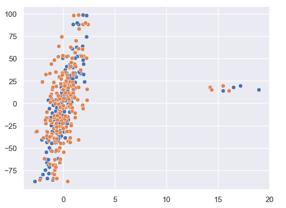
sns.scatterplot(x = X[:,1], y = y)
sns.scatterplot(x = X[:,0], y = y)
As we can see from our data plotted that there are a few outliers in this. Let us see how Huber Regression and Linear Regression perform.
huber = HuberRegressor().fit(X, y)

lr = LinearRegression()
lr.fit(X,y)

print(f'True coefficients are {coef}')
>>>True coefficients are [20.4923687  34.16981149]
print(f'Huber coefficients are {huber.coef_}')
>>>Huber coefficients are [17.79064252 31.01066091]
print(f'Linear coefficients are {lr.coef_}')
>>>Linear coefficients are [-1.92210833  7.02266092]
Here we can see that the Huber coefficients are closer to the true coefficients, let us also visualise this by plotting the line.
# use line_kws to set line label for legend

fig, axes = plt.subplots(nrows=1, ncols=2, figsize=(10, 5))
sns.regplot(x=X[:,1], y=y, color='b',
 line_kws={'label':"y={0:.1f}x+{1:.1f}".format(huber.coef_[1],huber.intercept_)}, ax = axes[0])
axes[1] = sns.regplot(x=X[:,1], y=y, color='r',
 line_kws={'label':"y={0:.1f}x+{1:.1f}".format(lr.coef_[1],lr.intercept_)}, ax = axes[1])
In these plots, we can clearly see the effect the outlier has on the regression output between Linear and Huber Regression.
MSLE (Mean Squared Logarithmic Error) and MSE (Mean Squared Error) are both loss functions that you can use in regression problems. But when should you use what metric?
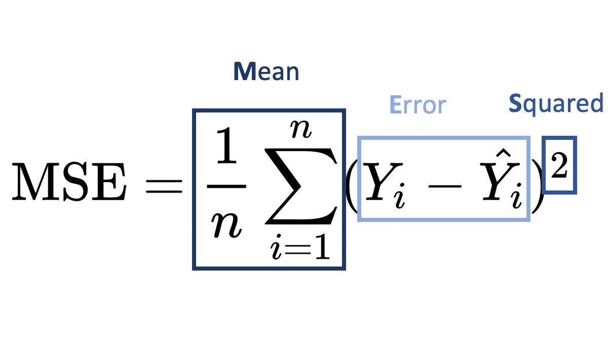
Mean Squared Error (MSE):
It is useful when your target has a normal or normal-like distribution, as it is sensitive to outliers.
An example is below –
In this case using MSE as your loss function makes much more sense than MSLE.
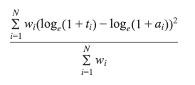
Mean Squared Logarithmic Error (MSLE):
MSLE measures the average squared logarithmic difference between the predicted and actual values.
MSLE treats smaller errors as less significant than larger ones due to the logarithmic transformation.
It is less sensitive to outliers than MSE since the logarithmic transformation compresses the error values.
An example where you can use MSLE –
Here if you use MSE then due to the exponential nature of the target, it will be sensitive to outliers and MSLE is a better metric, remember that MSLE cannot be used for optimisation, it is only an evaluation metric.
In general, the choice between MSLE and MSE depends on the nature of the problem, the distribution of errors, and the desired behavior of the model. It’s often a good idea to experiment with both and evaluate their performance using appropriate evaluation metrics before finalizing the choice.
In this series of posts, I’ll be covering how to approach time series forecasting in python in detail. We will start with the basics and build on top of it. All posts will contain a practice example attached as a GitHub Gist. You can either read the post or watch the explainer Youtube video below.
# Loading Libraries
import numpy as np
import pandas as pd
import seaborn as sns
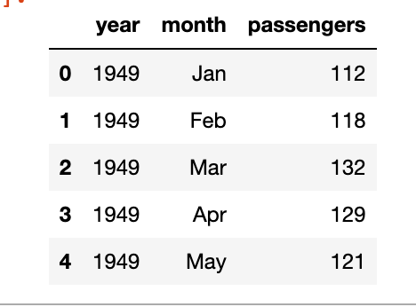
We will be using a simple linear regression to predict the outcome of the number of flights in the month of May. The data is taken from seaborn datasets.
As you can see we’ve the year, the month and the number of passengers, as a dummy example we will focus on the number of passengers in the month of May, below is the plot of year vs passengers.
We can clearly see a pattern here and can build a simple linear regression model to predict the number of passengers in the month of May in future years. The model will be like y = slope * feature + intercept. The feature, in this case, will be the number of passengers but shifted by 1 year. Meaning the number of passengers in the year 1949 will be the feature for the year 1950 and so on.
We can see that the p-value of the feature is significant, the intercept is not so significant, and the R-squared value is 0.97 which is very good. Of course, this is a dummy example so the values will be good.
df['prediction'] = df['lag_1']*m + b
sns.lineplot(x='year', y='value', hue='variable',
             data=pd.melt(df, ['year']))
One often thinks that you can use deep learning for classification problems like text or image classification, or for similar tasks like segmentation, language models etc. But you can also do simple linear regression with deep learning libraries. I’ve also attached the GitHub Gist in case you want to explore the working notebook.
In this post I’ll go over the model, it’s explanation on how can you do linear regression with keras.
In Keras, it can be implemented using the Sequential model and the Dense layer. Here’s an example of how to implement linear regression with Keras:
First we take a toy regression problem from scikit-learn datasets.
from sklearn.datasets import load_diabetes
from sklearn.model_selection import train_test_split

X,y = load_diabetes(return_X_y=True)

X_train, X_test, y_train, y_test = train_test_split(X,y, train_size=0.8)
Now we will need to define the model using Keras. That is actually very simple, you just have to take one sequential model with a Dense layer. The activation for this layer will be linear as we’re building a linear model and the loss will be mean squared error.
import numpy as np
from keras.models import Sequential
from keras.layers import Dense

# define the model
model = Sequential()
model.add(Dense(units=1, activation='linear'))
# compile the model
model.compile(optimizer='sgd', loss='mean_squared_error', metrics = ['mae'])

#fit the model
model.fit(x=X_train, y=y_train, validation_data=(X_test,y_test),
          epochs=100, batch_size=128)
Thats then all that is left is to call model.predict(X_test).
I was going through Kaggle competitions when this competition caught my eye, especially the evaluation metric for it. Now the usual metrics for forecasting or regression problems are either or , but sMAPE is different.
SMAPE (Symmetric Mean Absolute Percentage Error) is a metric that is used to evaluate the accuracy of a forecast model. It is calculated as the average of the absolute percentage differences between the forecasted and actual values, with the percentage computed using the actual value as the base. Mathematically, it can be expressed as:
So when to use which metric ?
RMSE – When you want to penalize large outlier errors in your prediction model, RMSE is the metric of choice as it penalizes large errors more than smaller ones.
MAPE – All errors have to be treated equally, so in those cases MAPE makes sense to use
sMAPE – is typically used when the forecasted values and the actual values are both positive, and when the forecasts and actuals are of similar magnitudes. It is symmetric in that it treats over-forecasting and under-forecasting the same.
It is important to note that in both MAPE and sMAPE, values of 0 are not allowed for both actual and forecast values as it would result in division by zero error.
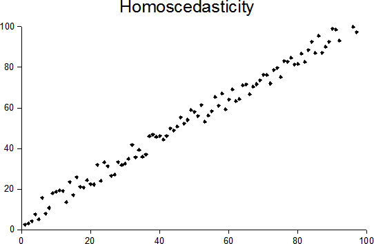
Once your linear regression model is trained, you should always plot your residuals (y – ŷ) whether the errors are homoscedastic or heteroscedastic. What do we mean by these terms? It means that there should not be any pattern in residuals and they should be uniformly distributed, or in other words, there should not be any variance in the residuals. Homoscedasticity is one of the assumptions of linear regression, so it is often important to check for it.
source: Wikipedia
source: Wikipedia
In the above figures, you can clearly see that the residuals have a clear pattern in the heteroscedastic image. In that scenario, you cannot rely on the regression analysis.
How to test for heteroscedasticity?
There are many ways to test for heteroscedasticity, I’ll list a. few ways here –
Visual Test – Just look at the residual plot and you’ll often see whether the residuals have any variance or not, not very accurate but often works.
Bartlett test
Breusch Pagan test
Goldfeld Quandt test
Glesjer test
Test based on Spearman’s rank correlation coefficient
White test
Ramsey test
Harvey Phillips test
Szroeter test
Peak test (nonparametric) test
All these tests in one way or another try to reject the null hypothesis H0 : variance is constant and the alternative hypothesis is that Ha : variance is not constant. You can go into detail about the tests here.
Variance Inflation Factor (VIF) determines the multicollinearity amongst the independent variables (predictors). Multicollinearity is when there is a high correlation between your predictor variables, usually 0.8 or higher. This can adversely affect your regression analysis.
How is it calculated?
VIF of a predictor variable is calculated by regressing it against all other predictor variables. This gives the R2 value which can be plugged into this formula
This will give the VIF value of a predictor.
VIF = 1, not correlated
VIF < 5, slightly correlated
VIF > 5, highly correlated
These values are just guidelines and how high acceptable VIF values are depends on the problem statement.
If you don’t want to use VIF and have very few predictor variables, one can plot a correlation matrix and remove the highly correlated variables.
You might also wonder why do we calculate the p-value of predictor variables in Linear regression. Find out why here.
Ever wondered why we look for p-value less than 0.05 for the coefficients when looking at the linear regression results.
Let’s quickly recap the basics of linear regression. In Linear Regression we try to estimate a best fit line for given data points. In case we have only one predictor variable and a target the linear equation will look something like
Y = A + Bx
Here A being the intercept and B being the slope or coefficient.
The null hypothesis for linear regression is that B=0 and the alternate hypothesis is that B != 0.
This is the reason why we look for p-value < 0.05 to reject the null hypothesis and establish that there exists a relationship between the target and the predictor variable.


 or
or  , but sMAPE is different.