Category: ML

  • Imblearn – The Python package to deal with Imbalanced Classes.

    NOTE – The article is under progress, I’ll be uploading the Youtube and linking the Kaggle notebook soon.

    Most often the data you get in the real world for classification tasks is imbalanced. You always end up dealing with the imbalance on your own before passing it through models, but what if there was a python package, built on top of scikit-learn that could do the heavy lifting for you, that’s exactly what imbalanced-learn (imblearn) is.

    I was inspired to use this package due this Kaggle Competition. I’ve linked the notebook in this post so you can refer it.
    But I’ll highly encourage you to watch the Youtube video below where I go over how I leverage imblearn with XgBoost to get a very good and balanced model as a baseline with very little effort.

    There are many ways imblearn which you can leverage to balance your data.

    The first is Synthetic Minority Oversampling Technique (SMOTE)

    To use this, all you have to do is to invoke the following code below –

    from imblearn.over_sampling import SMOTE, ADASYN
    X_smote, y_smote = SMOTE().fit_resample(X, y)
    

    After this your minortity class will up-sampled. There are also variations of SMOTE which you can use to balance your data using the library.

    Similarly you can call X_adasyn, adasyn = ADASYN().fit_resample(X,y) to oversample your data.

    There is also another function which will balance your data, but do know that this will take a lot of time to execute, and that is SMOTEENN (Over-sampling using SMOTE and cleaning using ENN).

    To call this you again have to use these two lines of code and let imblearn do the heavy lifting for you.

    from imblearn.combine import SMOTEENN
    X_balanced, y_balanced = SMOTEENN().fit_resample(X,y)
    

    You can also use any one of the following methods to undersample your data, note that undersampling using k-nearest neighbour methods will take some time.

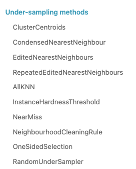
    Again all you have to do is use <undersampling method>.fit_resample(X,y)

    Once your data is ready, you can tune your model. The best thing about the competition was that the features were generated through some sort of PCA transformation, so we could easily use techniques like SMOTE, ADASYN to train the models. I did not use SMOTEENN as the notebook on Kaggle started to time out.

    Here is the link to the starter notebook, you can play around with it and try other sampling methods in imblearn.

    Hopefully, this post gave you insights on leveraging imblearn in your imbalanced classification problems.

  • ML Metrics | Top N Accuracy Explained

    This metric is usually used in multiclass classification problems.
    Each multiclass model gives a probability score for all the classes it is being trained on, but often you take the highest one, by using np.argmax but what if you took the top n classes and gave credit to the model if it got right in one of the n predictions.
    That is what is top n accuracy, it gives the model more chances to be right.

    Lets take an example.

    Suppose you built a model that predicts 3 classes and you want to find the top 2 accuracy of your model.
    Then you would pass the prediction array to the model and the true values and if the correct prediction is in the top 2 then you give it credit for being right.

    import numpy as np
    from sklearn.metrics import top_k_accuracy_score
    y_true = [0,1,1,2,2]
    y_pred = [[0.25, 0.2,0.3], #Here 0 is in the top 2
              [0.3, 0.35, 0.5], #Here 1 is in the top 2
              [0.2,0.4, 0.45], #Here 1 is in the top 2
              [0.5, 0.1, 0.2], #Here 2 is in the top 2
              [0.1, 0.4, 0.2]] #Here 2 is in the top 2
    top_k_accuracy_score(y_true, y_pred, k=2)
    

    It is 1.0, because the correct class was always in our top 2 prediction, actually, if you notice then it was always the second prediction of our model, so if we take regular accuracy or set the value k = 1 in top_k_accuracy_score(y_true, y_pred, k=2), the answer is 0.

    Hopefully, this explains what top N accuracy is, and if you want me to cover any ML topic, write in the comments below. Thanks for reading.

  • 5 Essential Boosting Parameters You Should Be Tuning

    Here are the 5 essential hyper-parameters that you should be always tuning when building any boosting model, whether you’re using XgBoost, LightGBM or even CatBoost.

    1. n_estimators – It is not the number of trees that the boosting algorithm will grow, but as the name suggests, the number of times gradient boosting will occur, so if you are using a tree-based boosting algorithm, then if you make this number 5, then each round of boosting fits a single tree to the negative gradient of some loss function.
    2. max_depth – The depth of each tree, pretty simple, the higher this number, the stronger each learner is in the model and the more your model can overfit. So pretty important to tune.
    3. learning_rate – Again a very important param, the higher it is the faster your algorithm will converge to the local minima, but too high and it might overshoot the minima, too low and it might never reach the minima.
    4. subsample – Sample of the training data to be used in each boosting round, if you use 0.5, then xgboost will randomly sample half your training data in each boosting iteration before growing the tree. Important if you want to control overfitting.
    5. colsample_bytree – Fraction of columns to use when growing a tree, again if set to 0.5, xgboost will randomly sample half of your features to grow the tree in each boosting round. Again very important to control overfitting.

    In another post I’ll be going over another 5 essential hyper-parameters that you should be tuning.

  • Time Series Forecasting with Python – Part 1 (Simple Linear Regression)

    In this series of posts, I’ll be covering how to approach time series forecasting in python in detail. We will start with the basics and build on top of it. All posts will contain a practice example attached as a GitHub Gist. You can either read the post or watch the explainer Youtube video below.

    # Loading Libraries
    import numpy as np
    import pandas as pd
    import seaborn as sns
    

    We will be using a simple linear regression to predict the outcome of the number of flights in the month of May. The data is taken from seaborn datasets.

    sns.set_theme()
    flights = sns.load_dataset("flights")
    flights.head()
    

    As you can see we’ve the year, the month and the number of passengers, as a dummy example we will focus on the number of passengers in the month of May, below is the plot of year vs passengers.

    We can clearly see a pattern here and can build a simple linear regression model to predict the number of passengers in the month of May in future years. The model will be like y = slope * feature + intercept. The feature, in this case, will be the number of passengers but shifted by 1 year. Meaning the number of passengers in the year 1949 will be the feature for the year 1950 and so on.

    df = flights[flights.month == 'May'][['year', 'passengers']]
    df['lag_1'] = df['passengers'].shift(1)
    df.dropna(inplace = True)
    

    Now we have the feature, let’s build the model-

    import statsmodels.api as sm
    y = df['passengers']
    x = df['lag_1']
    model = sm.OLS(y, sm.add_constant(x))
    results = model.fit()
    b, m = results.params
    

    Looking at the results

    OLS Regression Results                            
    ==============================================================================
    Dep. Variable:             passengers   R-squared:                       0.969
    Model:                            OLS   Adj. R-squared:                  0.965
    Method:                 Least Squares   F-statistic:                     279.4
    Date:                Fri, 20 Jan 2023   Prob (F-statistic):           4.39e-08
    Time:                        17:52:21   Log-Likelihood:                -47.674
    No. Observations:                  11   AIC:                             99.35
    Df Residuals:                       9   BIC:                             100.1
    Df Model:                           1                                         
    Covariance Type:            nonrobust                                         
    ==============================================================================
                     coef    std err          t      P>|t|      [0.025      0.975]
    ------------------------------------------------------------------------------
    const         13.5750     17.394      0.780      0.455     -25.773      52.923
    lag_1          1.0723      0.064     16.716      0.000       0.927       1.217
    ==============================================================================
    Omnibus:                        2.131   Durbin-Watson:                   2.985
    Prob(Omnibus):                  0.345   Jarque-Bera (JB):                1.039
    Skew:                          -0.365   Prob(JB):                        0.595
    Kurtosis:                       1.683   Cond. No.                         767.
    ==============================================================================
    

    We can see that the p-value of the feature is significant, the intercept is not so significant, and the R-squared value is 0.97 which is very good. Of course, this is a dummy example so the values will be good.

    df['prediction'] = df['lag_1']*m + b
    sns.lineplot(x='year', y='value', hue='variable', 
                 data=pd.melt(df, ['year']))


    The notebook is uploaded as a GitHub Gist –

    Loading
    Sorry, something went wrong. Reload?
    Sorry, we cannot display this file.
    Sorry, this file is invalid so it cannot be displayed.
  • Weight of Evidence Encoding

    So today I was participating in this Kaggle competition and the data had too many categorical variables. One way to build a model with too many categorical variables is to use a model like Catboost and let it deal with encoding categorical variables. But I wanted to ensemble my results with an Xgboost model, so I had to encode them. Using the weight of evidence encoding, I got a solution which was a top 10 solution when submitted. I have made the notebook public, you can go here and see it.

    So what is weight of evidence ?

    To put it simply –

    woe = ln(\frac{percnegatives}{percpositives}) = ln(\frac{\frac{neggroup}{totalneg}}{\frac{posgroup}{totalpos}})

    I’ve gone through an example explaining the weight of evidence in the youtube video below.

  • Linear Regression with Keras

    One often thinks that you can use deep learning for classification problems like text or image classification, or for similar tasks like segmentation, language models etc. But you can also do simple linear regression with deep learning libraries. I’ve also attached the GitHub Gist in case you want to explore the working notebook.

    In this post I’ll go over the model, it’s explanation on how can you do linear regression with keras.

    In Keras, it can be implemented using the Sequential model and the Dense layer. Here’s an example of how to implement linear regression with Keras:

    First we take a toy regression problem from scikit-learn datasets.

    from sklearn.datasets import load_diabetes
    from sklearn.model_selection import train_test_split
    
    X,y = load_diabetes(return_X_y=True)
    
    X_train, X_test, y_train, y_test = train_test_split(X,y, train_size=0.8)
    

    Now we will need to define the model using Keras. That is actually very simple, you just have to take one sequential model with a Dense layer. The activation for this layer will be linear as we’re building a linear model and the loss will be mean squared error.

    import numpy as np
    from keras.models import Sequential
    from keras.layers import Dense
    
    # define the model
    model = Sequential()
    model.add(Dense(units=1, activation='linear'))
    # compile the model
    model.compile(optimizer='sgd', loss='mean_squared_error', metrics = ['mae'])
    
    #fit the model
    model.fit(x=X_train, y=y_train, validation_data=(X_test,y_test), 
              epochs=100, batch_size=128)
    

    Thats then all that is left is to call model.predict(X_test).

    You can find the GitHub Gist below.

    Loading
    Sorry, something went wrong. Reload?
    Sorry, we cannot display this file.
    Sorry, this file is invalid so it cannot be displayed.
  • Information Gain, Gini and Decision Tree made from scratch

    In this post, we will go over the complete decision tree theory and also build a very basic decision tree using information gain from scratch.

    The below jupyter notebook as a Github Gist shows all the explanations and steps, including how to calculate Gini, Information gain and building a decision tree using the information gain you calculate.

    You can also watch the video explainer here on youtube.

    Loading
    Sorry, something went wrong. Reload?
    Sorry, we cannot display this file.
    Sorry, this file is invalid so it cannot be displayed.
  • Random Projection, how it is different from PCA and where is it used

    Random projection is another dimensionality reduction algorithm like PCA, as the name suggests, the basic idea behind Random Projection is to map the original high-dimensional data onto a lower-dimensional space while preserving as much of the pairwise distances between the data points as possible. This is done by generating a random matrix of size (n x k) where n is the dimensionality of the original data and k is the desired dimensionality of the reduced data.

    If we have a matrix M of dimension mxn and another matrix R of dimension nxk whose columns are representing random directions, the random projection of M is then calculated as

    M_{p} = MR

    The idea behind random projection is similar to PCA, but in PCA we first compute the eigenvalues, here we project the vector on random directions without any complex computations.

    The random matrix used for the projection can be generated in a variety of ways. One popular method is the Johnson-Lindenstrauss lemma, which states that the pairwise distances between the points in the original space can be approximately preserved if the dimensionality of the lower-dimensional space is chosen to be logarithmic in the number of data points. Another popular method is the use of random gaussian matrix.

    The Gaussian random projection reduces the dimensionality by projecting the original input space on a randomly generated matrix where components are drawn from the following distribution N(0, \frac{1}{n_{components}}).

    Why use Random Projection in place of PCA ?

    Random Projection is often used in large-scale data analysis and machine learning applications where computational resources are limited and the dimensionality of the data is too high. In such cases, calculating PCA is often too time-consuming and computationally expensive. Additionally, Random Projection is less sensitive to the presence of noise and outliers in the data compared to PCA.

  • LeetCode #11 – Container With Most Water

    Sometimes, coding questions are also part of data science interviews, so here is the solution to LeetCode #11 – the container with the most water problem.

    The problem is very straightforward, you’re given a list with n integers, each representing the height of a tower, you’ve to find the maximum area that can be formed with these heights and the x-axis represents the index distance between the integers with a twist that since it represents a block containing water, you’ve to take the min of the two heights as the water has to contained within the towers.

    For example, if the list of given heights is h = [1,1,4,5,10,1], the maximum area that can be formed will be 8. It will be between the tower with heights 4 and 10, with an index distance of 2. So the area will be min(4,10)*2 = 8.

    Coming to the solution, the easiest solution will be to compare each combination of two tower heights, and return the maximum area that can be formed. This will have a time complexity of O(n^{2})

    def maxArea(height: List[int]) -> int:
            max_vol = 0
            for i in range(len(height)):
                for j in range(1,len(height)):
                    if j<=i:
                        continue
                    else:
                        vol = min(height[i], height[j])*(j-i)
                        max_vol = max(max_vol, vol)
            return max_vol
    

    Although the above solution will pass the sample test cases, it will eventually return Time Limit Exceeded as it is a very brute force solution, as it compares almost every possible combination. You can be a bit more clever in your approach and solve this problem in O(n) time complexity.

    The trick is using pointers, one for left and one for right, starting with the largest width and then storing the max area. Move the left pointer right if you encounter a higher tower in the left otherwise move the right pointer towards the left, and repeat till both pointers meet. In this way, you’ve traversed the list only once.

    def maxArea(height: List[int]) -> int:
            l,r = 0,len(height) - 1
            max_vol = -1
            while l < r:
                #Calculating the shorter height of the two
                shorter_height = min(height[l], height[r])
                width = r-l
                vol = shorter_height * width
                max_vol = max(vol, max_vol)
                if height[l] < height[r]:
                    l+=1
                else:
                    r-=1
            return max_vol
    

    Taking an example, if input is [1,4,5,7,4,1], then.

    Steplrwidthmin heightareamax area
    1055155
    2044145
    314341212
    41324812
    52315512
    The loop will exit after step 5 as in step 6 l = r = 3, and we get the max area as 12.

  • sMAPE vs MAPE vs RMSE, when to use which regression metric

    I was going through Kaggle competitions when this competition caught my eye, especially the evaluation metric for it. Now the usual metrics for forecasting or regression problems are either RMSE = \sqrt{\frac{\sum (y - \hat{y})^{2}}{N}} or MAPE = \frac{1}{N}\sum_{t=1}^{n}\frac{\left|A_{t}-F_{t}\right|}{\left|A_{t}\right|}, but sMAPE is different.

    SMAPE (Symmetric Mean Absolute Percentage Error) is a metric that is used to evaluate the accuracy of a forecast model. It is calculated as the average of the absolute percentage differences between the forecasted and actual values, with the percentage computed using the actual value as the base. Mathematically, it can be expressed as:

    sMAPE = \frac{100}{n}\sum_{t=1}^{n}\frac{\left|F_{t} - A_{t} \right|}{(\left|A_{t} \right| + \left|F_{t} \right|)/2}

    So when to use which metric ?

    • RMSE – When you want to penalize large outlier errors in your prediction model, RMSE is the metric of choice as it penalizes large errors more than smaller ones.
    • MAPE – All errors have to be treated equally, so in those cases MAPE makes sense to use
    • sMAPE – is typically used when the forecasted values and the actual values are both positive, and when the forecasts and actuals are of similar magnitudes. It is symmetric in that it treats over-forecasting and under-forecasting the same.

    It is important to note that in both MAPE and sMAPE, values of 0 are not allowed for both actual and forecast values as it would result in division by zero error.