Category: Python

How To Calculate Correlation Among Categorical Variables?
We know that calculating the correlation between numerical variables is very easy, all you have to do is call df.corr().

But how do you calculate the correlation between categorical variables?

If you have two categorical variables then the strength of the relationship can be found by using Chi-Squared Test for independence.

The Chi-square test finds the probability of a Null hypothesis (H0).

Assumption(H0): The two columns are not correlated. H1: The two columns are correlated. Result of Chi-Sq Test: The Probability of H0 being True

We will be using the titanic dataset to calculate the chi-squared test for independence on a couple of categorical variables.
```
import numpy as np
import pandas as pd
import seaborn as sns
from matplotlib import pyplot as plt

df = sns.load_dataset('titanic')
corr = df[['age', 'fare', 'pclass']].corr()

# Generate a mask for the upper triangle
mask = np.triu(np.ones_like(corr, dtype=bool))

# Set up the matplotlib figure
f, ax = plt.subplots(figsize=(11, 9))

# Generate a custom diverging colormap
cmap = sns.diverging_palette(230, 20, as_cmap=True)

# Draw the heatmap with the mask and correct aspect ratio
sns.heatmap(corr, mask=mask, cmap=cmap, vmax=.3, center=0,
            square=True, linewidths=.5, cbar_kws={"shrink": .5})
```
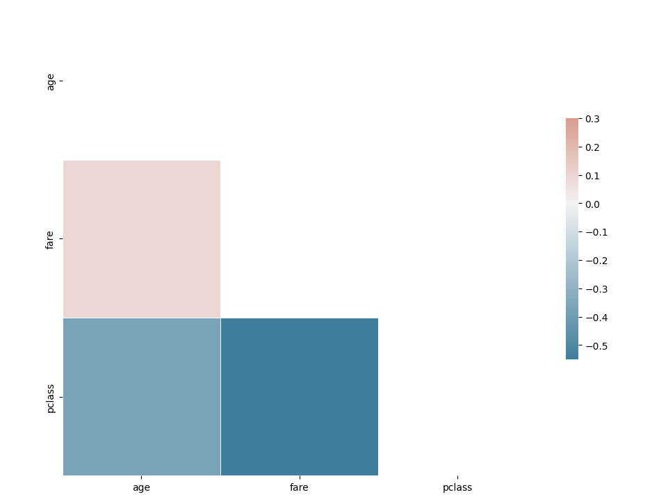
Pretty easy to calculate the correlation among numerical variables.

Lets first calculate first whether the class of the passenger and whether or not they survive have a correlation.
```
# importing the required function
from scipy.stats import chi2_contingency
cross_tab=pd.crosstab(index=df['class'],columns=df['survived'])
print(cross_tab)
```
```
chi_sq_result = chi2_contingency(cross_tab,)
p, x = chi_sq_result[1], "reject" if chi_sq_result[1] < 0.05 else "accept"

print(f"The p-value is {chi_sq_result[1]} and hence we {x} the null Hpothesis with {chi_sq_result[2]} degrees of freedom")
```
```
The p-value is 4.549251711298793e-23 and hence we reject the null Hpothesis with 2 degrees of freedom
```
Similarly, we can calculate whether two categorical variables are correlated amongst other variables as well.

Hopefully, this clears up how you can calculate whether two categorical variables are correlated or not in python. In case you have any questions please feel free to ask them in the comments.
January 23, 2023
Elo Rating – How to match with an opponent with equal strength.
Well, the Tata Steel Chess Tournament is going on in the Netherlands, where the best Chess Players in the world, including Magnus Carlsen, are playing. They have insane chess ratings like Ding and Carlsen are rated 2800+ while the lowest rated player is 2681. Now that is some tough competition. With my measly rating of around 1200, I would not stand a chance. But the question remains, how do you come up with these ratings?

This question must have also perplexed Arpad Elo, the inventor of the Elo rating system. It tries to measure the relative skill of players in zero-sum games such as Chess. A zero-sum game is just a fancy word for saying a game where one side loses and the other side wins, or it is a draw, it cannot happen that both sides walk away with an advantageous result.

How to Calculate it?

Support player A has a rating of R_A and player B has a rating of R_B. Then we calculate the expected probability of a win for each of the players using the formula –

$P_{A} = \frac{1}{1+{10^{(R_{B}-R_{A})/400}}}$

$P_{B} = \frac{1}{1+{10^{(R_{A}-R_{B})/400}}}$

After the match player A scores S_Apoints then we will update his rating according to the formula –

$R_{A}^{new} = R_{A} + k(S_{A} - P_{A})$ where the k-factor determines how the rating reacts to new results. If the value is set too high the ratings will jump around too much and if set too low it will take a long time to recognize greatness.

Let’s take an example. If Magnus plays against Fabi, then
```
#Function to calculate expected points

def expected_points(x,y):
    return 1/(1+10**((y-x)/400))

#Live ratings
r_magnus = 2850
r_fabi = 2768

#Expected points
e_magnus = expected_points(r_magnus, r_fabi)
e_fabi = expected_points(r_fabi, r_magnus)
#e_magnus = 0.615864104253756
#e_fabi = 0.384135895746244)
# If we assume that fabi wins, and a k-factor of 16, then

def new_rating(rating, k, points, expected_points):
    return rating + k*(points - expected_points)

magnus_new_rating = new_rating(r_magnus, 16, 0, e_magnus)
fabi_new_rating = new_rating(r_fabi, 16, 1, e_fabi)
```
Once you do the calculation, you will see that Magnus’s rating is 2840 and Fabi’s rating is now 2777.

Had Fabi lost, his rating would not go down as drastically as Magnus’s did when he lost, for example, if Fabi lost in this example, his rating will be 2761.85, so he lost lesser points when losing to a higher-rated opponent, but gains a lot if he manages to beat one. Spoiler alert – Fabi lost against Magnus in the Tata Steel Chess Tournament.

Hopefully, this post made it a bit clear how you can calculate Elo Ratings and how are they calculated for Chess Players. Fun fact, these ratings are calculated behind the scenes of almost every multi-player game to ensure that they always match you to an opponent of similar skill.
January 23, 2023
Pandas Essentials – Pivot, Pivot Table, Cast and Melt
How to transform your data to generate insights is one of the most essential skills a Data Scientist can have. Knowing state-of-the-art models will be of no use if you cannot transform your data with ease. Pandas is a data manipulation library in python that everyone knows. It is so ubiquitous that all of us starting off in Data Science start our notebooks with import pandas as pd.

In this post, we will go over some pandas skills that many people either don’t know, don’t use or find difficult to understand.

As usual, you can either read the post or watch the Youtube video below.

We will be using the flights data from seaborn as an example to go over.
```
import pandas as pd
import numpy as np
import seaborn as sns
flights = sns.load_dataset('flights')
flights.head()
```
Pivot and Pivot Table

Now suppose that you want to create a table which had year as rows and month as columns and the passengers as values, then you will use pivot. Here is the pivot function from the official documentation of pandas – DataFrame.pivot(*, index=None, columns=None, values=None)

In this particular example, you’ll use year as index, month as columns and passengers in values.

flights.pivot(index='year', columns='month', values='passengers')

Now the most important question is why there is pivot and a pivot_table in pandas. The reason is that pivot only reshapes the data, it does not support data aggregation, for data aggregation you will have to use pivot_table.

Now suppose I wanted to create a table which will show me for every year, what was the maximum, minimum and mean number of passengers, then there are two ways I can do it, I can either use groupby or I can use pivot_table. Here is the official documentation from pandas for pivot_table. Note: You can pass multiple aggregation functions.

DataFrame.pivot_table(values=None, index=None, columns=None, aggfunc='mean', fill_value=None, margins=False, dropna=True, margins_name='All', observed=False, sort=True)

flights.pivot_table(values = 'passengers', index = 'year', aggfunc=[np.max, np.min, np.mean])

Melt

Melt is used to convert wide-form data into long-form, suppose we started with the flights data in its pivot form, that is –

flights_wide = flights.pivot(index='year', columns='month', values='passengers')

And we wanted to return to the flights data form, then melt can be thought of as the unpivot of pandas. To return to the original form you simply have to –

flights_wide.melt(value_name='passengers', ignore_index=False)

Here we don’t use an id_var as there is None, we add ignore_index as False as we want to return the index which has the year in it and we call the value_name as passengers.

As a recap, remember that pivot makes long-form data into wide-form and melt takes wide-form data and converts it into long-form data

So where is Cast in Pandas?

People who have used R as a programming language often ask where is the cast functionality in pandas, the pivot_table we saw earlier is pandas’s answer to the cast functionality in Python.
January 21, 2023
Weight of Evidence Encoding

So today I was participating in this Kaggle competition and the data had too many categorical variables. One way to build a model with too many categorical variables is to use a model like Catboost and let it deal with encoding categorical variables. But I wanted to ensemble my results with an Xgboost model, so I had to encode them. Using the weight of evidence encoding, I got a solution which was a top 10 solution when submitted. I have made the notebook public, you can go here and see it.

So what is weight of evidence ?

To put it simply –

$woe = ln(\frac{percnegatives}{percpositives}) = ln(\frac{\frac{neggroup}{totalneg}}{\frac{posgroup}{totalpos}})$

I’ve gone through an example explaining the weight of evidence in the youtube video below.

January 18, 2023
LeetCode #11 – Container With Most Water
Sometimes, coding questions are also part of data science interviews, so here is the solution to LeetCode #11 – the container with the most water problem.

The problem is very straightforward, you’re given a list with n integers, each representing the height of a tower, you’ve to find the maximum area that can be formed with these heights and the x-axis represents the index distance between the integers with a twist that since it represents a block containing water, you’ve to take the min of the two heights as the water has to contained within the towers.

For example, if the list of given heights is h = [1,1,4,5,10,1], the maximum area that can be formed will be 8. It will be between the tower with heights 4 and 10, with an index distance of 2. So the area will be min(4,10)*2 = 8.

Coming to the solution, the easiest solution will be to compare each combination of two tower heights, and return the maximum area that can be formed. This will have a time complexity of $O(n^{2})$
```
def maxArea(height: List[int]) -> int:
        max_vol = 0
        for i in range(len(height)):
            for j in range(1,len(height)):
                if j<=i:
                    continue
                else:
                    vol = min(height[i], height[j])*(j-i)
                    max_vol = max(max_vol, vol)
        return max_vol
```
Although the above solution will pass the sample test cases, it will eventually return Time Limit Exceeded as it is a very brute force solution, as it compares almost every possible combination. You can be a bit more clever in your approach and solve this problem in $O(n)$ time complexity.

The trick is using pointers, one for left and one for right, starting with the largest width and then storing the max area. Move the left pointer right if you encounter a higher tower in the left otherwise move the right pointer towards the left, and repeat till both pointers meet. In this way, you’ve traversed the list only once.
```
def maxArea(height: List[int]) -> int:
        l,r = 0,len(height) - 1
        max_vol = -1
        while l < r:
            #Calculating the shorter height of the two
            shorter_height = min(height[l], height[r])
            width = r-l
            vol = shorter_height * width
            max_vol = max(vol, max_vol)
            if height[l] < height[r]:
                l+=1
            else:
                r-=1
        return max_vol
```
Taking an example, if input is [1,4,5,7,4,1], then.

Step l r width min height area max area
1 0 5 5 1 5 5
2 0 4 4 1 4 5
3 1 4 3 4 12 12
4 1 3 2 4 8 12
5 2 3 1 5 5 12
The loop will exit after step 5 as in step 6 l = r = 3, and we get the max area as 12.
January 13, 2023