Tag: AI

An Illustrated Guide to Gradient Descent
How will you minimise this function –

$f(x) = x^{2}$

The mathematical solution will be to find the derivative, then solve the equation, $\frac{\partial f(x)}{\partial x} = 2x = 0$ , which gives the solution as x = 0. But what if you don’t know this and need to rely on a method which can reach the minimum of a function iteratively. That is what gradient descent does.

Gradient descent as the name suggests is like slowly descending down the mountain that is the loss function but in an iterative manner. We always take a small step in the opposite direction of the gradient. If the gradient is positive, we take a negative step and if the gradient is negative then we take a positive step.

So in this example suppose we have to minimise $x^{2}$ and we start off with an initial value say 7. Then we we will update the value of x as –

x_new = x_old + (- $\frac{\partial f(x)}{\partial x}$ )*x_old*lr

where lr is the learning rate. Tuning this value is crucial is how fast we reach the minimum, or if we overshoot the minimum and never reach it.

Let’s take an example in python –
```
import matplotlib.pyplot as plt
import matplotlib.animation as animation
import numpy as np

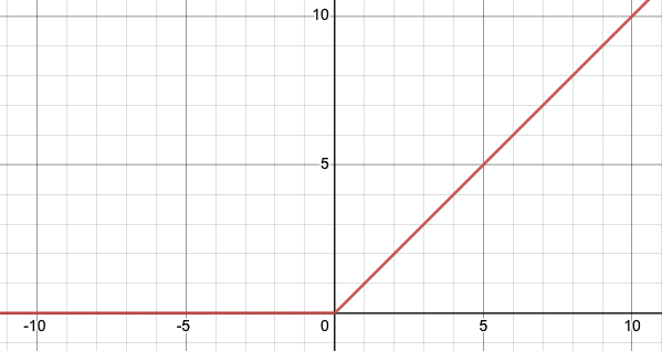
def f(x):
    return x**2

def derivative(x):
    return 2*x

y = [f(x) for x in np.arange(-20,20,0.2)]
x = np.arange(-20,20,0.2)

plt.plot(x,y)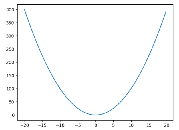
```
```
value = 7
lr = 0.1
derivatives = []
values = []
for i in range(9):
    values.append(value)
    derivatives.append(derivative(value))
    value = value - lr*derivative(value)

# List of points and derivatives
points = [(x,f(x)) for x in values]

# Create a 9x9 subplot grid
fig, axs = plt.subplots(3, 3, figsize=(9, 9))


# Plot the main plot (x^2) in the top-left subplot
axs[0, 0].plot(x, y, label='$x^2$', color='blue')
axs[0, 0].legend()

# Iterate over points and derivatives to create subplots
for i, (point_x, point_y) in enumerate(points):
    # Calculate the line passing through the point with the slope from the derivatives list
    slope = derivatives[i]
    line_y = x + slope * (x - point_x)

    axs[i//3, i%3].plot(x, y, color='blue')

    # Plot the point
    axs[i//3, i%3].plot(point_x, point_y, marker='x', markersize=10, color='red', label='Point')
    
    # Plot the line passing through the point with the specified slope
    axs[i//3, i%3].plot(x, line_y, linestyle='--', color='green', label=f'Slope = {slope}')

    # Set titles for subplots
    axs[i//3, i%3].set_title(f'Point at ({np.round(point_x,2)}, {np.round(point_y,2)})')

# Adjust layout for better visualization
plt.tight_layout()

# Show the plot
plt.show()
```
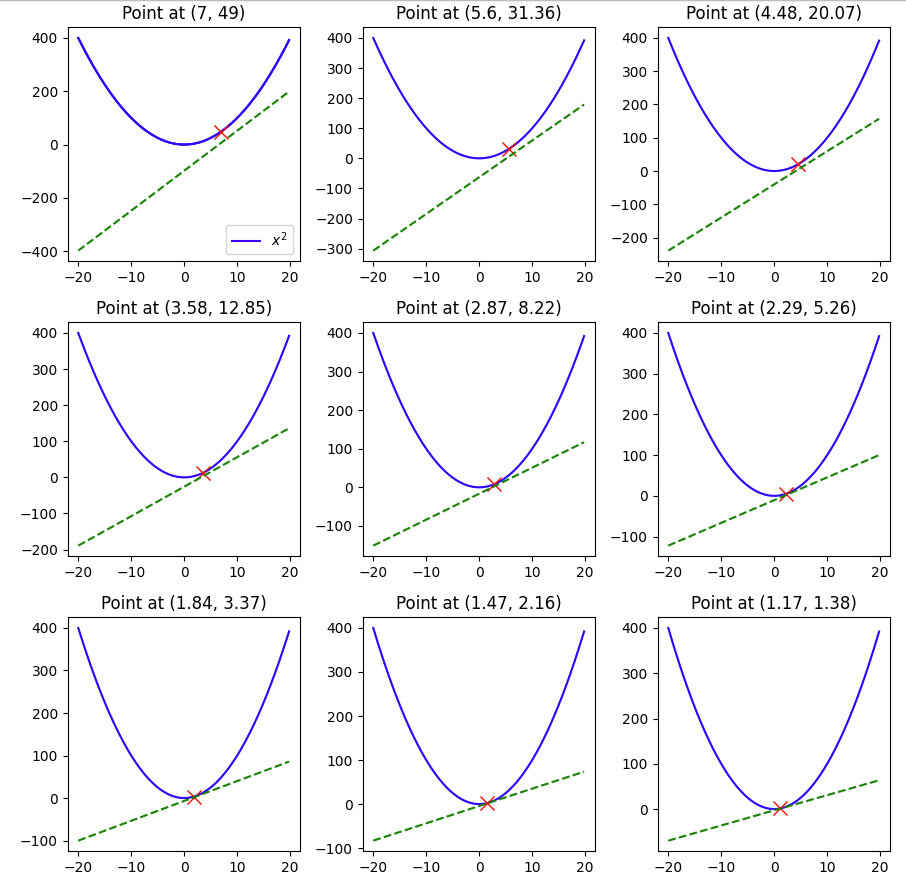
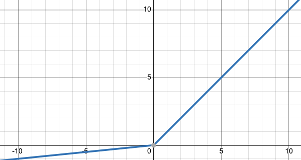
Here we see that with a learning rate of 0.1 and a starting value of 7 and in 9 steps we were able to reach 1.17, pretty close to the minimum of 0, but not quite so, if we change the lr to 0.3, let’s see what happens.

The minimum of 0 was reached within 9 steps.

But what happens if we make the lr 1 –

Here you can see that the value keeps oscillating between 7 and -7, and thus having a large learning rate also can be harmful when using ML models that use gradient descent.

Hopefully this example gave you a visual guide on how gradient descent works.
January 22, 2024

Custom Objective Function in XGBoost

In the previous post, we covered how you can create a custom loss function in Catboost, but you might be using catboost, so how can you create the same if you’re using Xgboost to train your models. In this post, I’ll walk over an example using the famous Titanic dataset, where we’ll recreate the LogLoss function and compare the results with the standard implementation in the library.

First, we have to set up the data.

import numpy as np 
import seaborn as sns
import pandas as pd
import xgboost as xgb
from sklearn.metrics import log_loss

data = sns.load_dataset('titanic')

Then some data cleaning and setting up the training dataset. The goal is not to get the best model but to demonstrate the custom loss function, so not much feature engineering is being done.

data['embarked'].fillna('S', inplace = True)

X,y = data[[c for c in data.columns if c not in  \
            ['survived', 'alive', 'deck', 'embark_town']]], \
      data['survived']

cat_columns = ['pclass', 'sex', 'sibsp', 'parch', 'embarked', 'class',
       'who', 'adult_male', 'alone']

X = pd.get_dummies(X, columns=cat_columns, drop_first=True)

Let’s say there was no loss function like logloss, then how would you define the logloss as an objective function.

$LogLoss = -1/N \sum({y_{i}log(\hat{y}) + (1-y_{i})log(1-\hat{y})})$

You’ll have to calculate the first and second derivative with respect to the $\hat{y}$

$\Large \frac{\partial LogLoss}{\partial \hat{y}} = -\frac{y_{i}}{\hat{y}} + \frac{1-y_{i}}{1-\hat{y}}$

$\Large \frac{\partial^2LogLoss }{\partial \hat{y}^2} = \frac{y_{i}}{\hat{y}^{2}} + \frac{1-y_{i}}{(1-\hat{y})^{2}}$

Now we will write these up as Python functions and create a function that returns the gradient and hessian (second derivative) values. In the xgboost library, the first value being passed is the predictions and the second is the training matrix.

def log_loss_derivative(y_pred, dtrain ):
    y = dtrain.get_label()
    return (-y/y_pred) + ((1-y)/(1-y_pred))

def log_loss_second_derivative(y_pred,  dtrain):
    y = dtrain.get_label()
    return (y/np.power(y_pred,2)) + ((1-y)/np.power((1-y_pred),2))

def custom_log_loss(predt, dtrain):
    y_pred = np.clip(predt, a_max=1-1e-5, a_min=1e-5)
    grad = log_loss_derivative(y_pred= y_pred, dtrain = dtrain)
    hess = log_loss_second_derivative(y_pred= y_pred, dtrain = dtrain)
    return grad, hess

We clip the predictions to avoid division by zero errors. Now let’s train.

import xgboost as xgb

dtrain =xgb.DMatrix(data=X, label=y)

model = xgb.train({'tree_method': 'hist', 'seed': 1994},
           dtrain=dtrain,
           num_boost_round=10,
           obj=custom_log_loss)

log_loss(y_pred=np.clip(model.predict(dtrain), a_max=1, a_min=0), y_true=y)
>>>0.24912

Comparison with the standard implementation.

clf = xgb.XGBClassifier(n_estimators = 10, **{'tree_method': 'hist', 'seed': 1994})
clf.fit(X,y)

log_loss(y_pred=np.clip(clf.predict_proba(X)[:,1], a_max=1, a_min=0), y_true=y)

>>>0.2861

As we can see the metrics are very close in our implementation of the LogLoss and the standard implementation. Of course, you should use the standard implementation when it’s available, but in case you want to use a custom loss function, you now know how to do so.

January 21, 2024

Creating a Custom Loss Function For Machine Learning Models

While standard Machine Learning Libraries provide a vast array of loss functions out of the box, sometimes we need to create our own custom loss function. In this blog post, I’ll go over a simple example and create a custom loss function in Catboost.

First we will create the data for training.

# Importing libraries
import numpy as np
import pandas as pd
from sklearn.metrics import mean_squared_error
from catboost import CatBoostRegressor, Pool
from sklearn.datasets import fetch_california_housing

raw_data = fetch_california_housing()

data = pd.concat([pd.DataFrame(raw_data['data'], columns=raw_data['feature_names']), 
                  pd.Series(raw_data['target'], name = 'target')], axis = 1)

features = [i for i in data.columns.tolist() if i != 'target']

Since the objective is not to create the best model possible, we won’t be doing any feature engineering. Let’s use catboost, and create a model using standard loss functions.

model = CatBoostRegressor(loss_function='RMSE', n_estimators=100, eval_metric='RMSE')

cb_pool = Pool(data=data[features], label=data['target'], feature_names=features)

model.fit(cb_pool)

predictions = model.predict(cb_pool)

mean_squared_error(y_true=data['target'], y_pred=predictions)

Upon evaluating the model we find that the mean squared error is 0.15. Definitely a model which is overfitting, but that’s not a concern for this tutorial.

But what is you don’t want to use RMSE as a loss function, and instead want to use something like this –

$loss = \frac{\sum (y - \hat{y})^{4}}{n}$

Then how do you create a loss function in catboost?

For this, you’ll need to calculate the first derivative and the second derivative of the loss function with respect to $\hat{y}$ .

Using the chain rule, the first derivative is

$\frac{\partial (y-\hat{y})^4}{\partial \hat{y}} = \frac{\partial (y-\hat{y})^4}{\partial (y-\hat{y})}*\frac{\partial y - \hat{y}}{\partial \hat{y}} = 4 * (y - \hat{y})^{3}* -1 = -4(y -\hat{y})^{3}$

And similarly using the chain rule, the second derivative comes out to be $12*(y-\hat{y})^2$

The catboost template for a custom objective is as follows –

class UserDefinedObjective(object):
    def calc_ders_range(self, approxes, targets, weights):
        """
        Computes first and second derivative of the loss function 
        with respect to the predicted value for each object.

        Parameters
        ----------
        approxes : indexed container of floats
            Current predictions for each object.

        targets : indexed container of floats
            Target values you provided with the dataset.

        weight : float, optional (default=None)
            Instance weight.

        Returns
        -------
            der1 : list-like object of float
            der2 : list-like object of float

        """
        pass

Using this temple, we can write the custom objective –

class CustomLossObjective(object):
    def calc_ders_range(self, approxes, targets, weights):
        assert len(approxes) == len(targets)
        if weights is not None:
            assert len(weights) == len(approxes)
        
        result = []
        n = len(targets)  # Number of samples

        for index in range(len(targets)):
            error = targets[index] - approxes[index]
            der1 = -4 * error**3
            der2 = 12 * error**2

            if weights is not None:
                der1 *= weights[index]
                der2 *= weights[index]

            result.append((der1, der2))
        return result

Now let’s use this custom loss in our model

model = CatBoostRegressor(loss_function=CustomLossObjective(), n_estimators=100, eval_metric='RMSE')
model.fit(cb_pool)

predictions = model.predict(cb_pool)
mean_squared_error(y_true=data['target'], y_pred=predictions)

Using this loss, we see that the mean squared error is 0.735, this is clearly inferior to using RMSE, but as mentioned before the objective of this blog post is not to build the best model but to showcase how one can create a custom loss objective in catboost.

January 14, 2024

GPT-4 Vision API – How to Guide

In the Dev Conference, OpenAI announced the GPT-4 Vision API. With access to this one can develop many tools, with the GPT-4-turbo model being the engine of your tool. The use cases can range from information retrieval to classification models.

In this article, we will go over how you can use the vision API, how can you pass multiple images with the API and some tricks you should be using to improve the response.

Firstly, you should have a billing account with OpenAI and also some credits to use this API, as, unlike ChatGPT, here you’re charged per token and not a flat fee, so be careful in your experiments.

The API –

The API consists of two parts –

Header – Here you pass your authentication key and if you want the organisation id
Payload – This is where the meat of your request lies. The image can be passed either as a URL or a base64 encoded image. I prefer to pass it in the latter way.

# To encode the image in base64

# Function to encode the image
def encode_image(image_path):
    with open(image_path, "rb") as image_file:
        return base64.b64encode(image_file.read()).decode('utf-8')

# Path to your image
image_path = "./sample.png"

# Getting the base64 string
base64_image = encode_image(image_path)

Let’s look at the API format

headers = {
    "Content-Type": "application/json",
    "Authorization": f"Bearer {API_KEY_HERE}"
}

payload = {
    "model": "gpt-4-vision-preview",
    "messages": [
         {"role": <user or system>,
          "content" : [{"type": <text or image_url>,
                        "text or image_url": <text or image_url>}]
}
    ],
    "max_tokens": <max tokens here>
}

response = requests.post("https://api.openai.com/v1/chat/completions", headers=headers, json=payload)

Let’s take an example.
Suppose I want to create a prompt which has a system prompt and a user prompt which can extract JSON output from an image. My payload will look like this.

payload = {
    "model": "gpt-4-vision-preview",
    "messages": [
# First define the system prompt        
{
        "role": "system",
        "content": [
            {
                "type": "text",
                "text": "You are a system that always extracts information from an image in a json_format"
            }
        ]
    },
        
    # Define the user prompt  
      {
        "role": "user",
# Under the user prompt, I pass two content, one text and one image
        "content": [
          {
            "type": "text",
            "text": """Extract the grades from this image in a structured format. Only return the output.
                       ```
                       [{"subject": "<subject>", "grade": "<grade>"}]
                       ```"""
          },
          {
            "type": "image_url",
            "image_url": {
              "url": f"data:image/jpeg;base64,{base64_image}"
            }
          }
        ]
      }
    ],
    "max_tokens": 500 # Return no more than 500 completion tokens
}

The return I get from the API is exactly how i wanted.

```json
[
  {"subject": "English", "grade": "A+"},
  {"subject": "Math", "grade": "B-"},
  {"subject": "Science", "grade": "B+"},
  {"subject": "History", "grade": "C+"}
]
```

This is just an example of how just by using the correct prompt we can built an information retrieval system on images using the vision API.

In the next article, we will build a classifier using the API, which will involve no knowledge of Machine Learning and just by using the API we will build a state-of-the-art image classifier.

November 11, 2023

I asked ChatGPT to write a language model

I asked ChatGPT to write a language model. Here is the code that it returned.

from keras.layers import Embedding, LSTM, Dense
from keras.models import Sequential

# Define the model
model = Sequential()
model.add(Embedding(input_dim=vocab_size, output_dim=embedding_size, input_length=max_length))
model.add(LSTM(units=hidden_size))
model.add(Dense(units=vocab_size, activation='softmax'))

# Compile the model
model.compile(optimizer='adam', loss='categorical_crossentropy')

# Fit the model to the training data
model.fit(x_train, y_train, batch_size=batch_size, epochs=num_epochs)

So I decided to build a language model using it, but before I had to write a couple of lines of code myself. First the Tokenizer.

class Tokenizer():
    def __init__(self, 
                 oov_token ='<unk>',
                 pad_token ='<pad>'):
        self.vocab = {}
        self.reverse_vocab = {}
        self.oov_token = oov_token
        self.pad_token = pad_token
        self.__add_to_dict(self.oov_token)
        self.__add_to_dict(self.pad_token)
        for i in range(10):
            self.__add_to_dict(str(i))
        for i in range(26):
            self.__add_to_dict(chr(ord('a') + i))

        # Add space and punctuation to the dictionary
        self.__add_to_dict('.')
        self.__add_to_dict(' ')
    
    def __add_to_dict(self, character):
        if character not in self.vocab:
            self.vocab[character] = len(self.vocab)
            self.reverse_vocab[self.vocab[character]] = character
        
    def tokenize(self, text):
        return [self.vocab[c] for c in text]

    def detokenize(self, text):
        return [self.reverse_vocab[c] for c in text]
    
    def get_vocabulary(self):
        return self.vocab
    
    def vocabulary_size(self):
        return len(self.vocab)
    
    def token_to_id(self,character):
        return self.vocab[character]
    
    def id_to_token(self , token):
        return self.reverse_vocab[token]
    
    def pad_seq(self,seq, max_len):
        return seq[:max_len] + [self.token_to_id(self.pad_token)]*(max_len-len(seq))

Then I added the config, created a small corpus of text and prepared the training data it needs to train the model. To prepare the training data I also asked how should the corpus be created and created the corpus as it showed me.

t = Tokenizer()
vocab_size = t.vocabulary_size()
embedding_size = 64
max_length = vocab_size
num_epochs = 50
batch_size = 16

corpus = ["this is a dog",
         "dogs live with humans", 
         "they are called what is known as pets",
         "cats are also pets",
         "there are also wolves in the jungle",
         "there are many animals in the jungle",
         "the lion is called the king of the jungle",
         "the largest animal in the jungle is the elephant",
         "we have horses also there",
         "foxes are quite quick and they are also very clever",
         "the zebra also looks like a horse but is not domesticated",
         "we go to the zoo to look at monkeys",
         "we all live together on this earth",
         'monkeys like bananas',
         'pandas eat bamboo',
         'tigers are dangerous',
         'zebras have stripes',
         'lions are the kings of the savannah',
         "it is upon humans to take care of this planet"]
tokenized_corpus = [t.tokenize(line) for line in corpus]
#Padding the tokenized corpus
x_train = np.array([t.pad_seq(sentence, max_length) for sentence in tokenized_corpus])

y_train = np.array([np.roll(sentence, -1) for sentence in x_train])

Also it had a mistake in the code, which I corrected, and ran the training loop. You can find the full code here on my Github.

I then asked ChatGPT to write the inference code for the model. Here is what it returned.

def generate_text(seed_text, model, max_gen_length, tokenizer):
    # Tokenize the seed text
    seed_text = tokenizer.tokenize(seed_text)
    # Pad the seed text to the maximum length
    seed_text = tokenizer.pad_seq(seed_text, max_length=30)
    # Initialize an empty list to store the generated words
    generated_text = []
    # Append the seed text to the generated text
    generated_text.extend(seed_text)
    # Loop for the specified number of words to generate
    for i in range(max_gen_length):
        # Use the model to predict the next word
        next_word_probs = model.predict(np.array([seed_text]))[0]
        # Get the index of the most probable next word
        next_word_idx = np.argmax(next_word_probs)
        # Append the generated word to the generated text
        generated_text.append(next_word_idx)
        # update the seed text
        seed_text = np.delete(seed_text, 0)
        seed_text = np.append(seed_text, next_word_idx)
    # Convert the generated text from indices to words
    generated_text = [tokenizer.id_to_token(word) for word in generated_text]
    return "".join(generated_text)

# Initialize the seed text
seed_text = "The sky is"
# Generate new text
generated_text = generate_text(seed_text, model, max_gen_length=10, tokenizer=tokenizer)
print(generated_text)

Making a few changes to the code to suit our tokenizer class and model, here are a few inputs and outputs.

Input - the sky is
Output - the sky is<pad><pad><pad><pad><pad><pad><pad><pad><pad><pad><pad><pad><pad><pad><pad><pad><pad><pad><pad><pad><pad><pad><pad><pad><pad><pad><pad><pad><pad><pad>4444444444
Input - "lion is the king of the jungle"
Output - lion is the king of the jungle<pad><pad><pad><pad><pad><pad><pad><pad><pad><pad>4444444444

Sure the output is terrible, but remember it is a very basic model architecture and we’ve not used transformers or temperature sampling to improve our language model. In my future posts, I’ll use ChatGPT to build upon these blocks to train even bigger and more complex language models.

This shows how ChatGPT or similar large language models can enable developers in writing code or develop models in a short amount of time. It is

January 15, 2023

ReLU vs Leaky ReLU, when to use what

ReLU (Rectified Linear Unit) and Leaky ReLU are both types of activation functions used in neural networks.

ReLU

ReLU is defined as f(x) = max(0, x), where x is the input to the function. It sets all negative input values to zero while allowing all non-negative values to pass through unchanged. This can help speed up training and improve the performance of the model because it reduces the number of negative input values that need to be processed by the model.

Leaky ReLU is an extension of ReLU that aims to address the problem of “dying ReLUs” in which some neurons in the network never activate because the gradient is zero for all input values less than zero. It can be defined mathematically as f(x) = max(x, kx) where k is usually a small negative slope (of 0.01 or so) for negative input values, rather than being zero as in a standard ReLU.

In practice, LeakyReLU is being used as a generalization of ReLU. This small negative slope helps in avoiding the dying ReLU problem. Also, it helps to train a network faster as the gradients for negative input values will not be zero. A general rule of thumb when choosing between the two would be that, if the problem does not have sparse inputs and the data set is not too small, using Leaky ReLU may result in a more accurate model. Otherwise, if the problem has sparse inputs and/or the data set is small, then using ReLU is a better choice.

It also depends on personal preferences and what the dataset is like. Sometimes leaky ReLU may work better in some cases and sometimes ReLU may be better. It’s important to try out different activation functions and see which one gives the best performance on your dataset.

January 11, 2023
Why Tanh is a better activation function than sigmoid ?
You might be asked that why often in neural networks, tanh is considered to be a better activation function than sigmoid.

Sigmoid

Tanh

Andrew NG also mentions in his deep learning specialization course that tanh is almost always a better activation function than sigmoid. So why is that the case?

There are a few reasons why the hyperbolic tangent (tanh) function is often considered to be a better activation function than the sigmoid function:
1. The output of the tanh function is centered around zero, which means that the negative inputs will be mapped to negative values and the positive inputs will be mapped to positive values. This makes the learning process of the network more stable.
2. The tanh function has a derivative that is well-behaved, meaning that it is relatively easy to compute and the gradient is relatively stable.
3. The sigmoid function, on the other hand, maps all inputs to values between 0 and 1. This can cause the network to become saturated, and the gradients can become very small, making the network difficult to train.
4. Another reason is that the range of the tanh function is [-1,1], while the range of the sigmoid function is [0,1], which makes the model output values more similar to the standard normal distribution. It will be less likely to saturate and more likely to have a good gradient flow, leading to faster convergence.
5. Another advantage is that the tanh function is differentiable at all points. In contrast, the sigmoid function has a kink at 0, which may cause issues when computing gradients during back-propagation, and other optimization methods.
All that being said, whether to use sigmoid or tanh depends on the specific problem and context, and it’s not always the case that one is clearly better than the other.
January 11, 2023
Null Hypothesis of Linear Regression Explained

Ever wondered why we look for p-value less than 0.05 for the coefficients when looking at the linear regression results.

Let’s quickly recap the basics of linear regression. In Linear Regression we try to estimate a best fit line for given data points. In case we have only one predictor variable and a target the linear equation will look something like

Y = A + Bx

Here A being the intercept and B being the slope or coefficient.

The null hypothesis for linear regression is that B=0 and the alternate hypothesis is that B != 0.

This is the reason why we look for p-value < 0.05 to reject the null hypothesis and establish that there exists a relationship between the target and the predictor variable.

January 5, 2023