Tag: Data Science Interview

  • What is MLaaS (Machine Learning as a Service)

    Like SaaS (Software as a Service), MLaaS is a cloud-based offering that allows users to access and utilize machine learning capabilities without needing to invest in the underlying infrastructure or have extensive expertise in machine learning. With MLaaS, users can access pre-built machine learning models, algorithms, and tools through APIs or web interfaces, enabling them to integrate machine learning capabilities into their applications, processes, or products. This approach simplifies the deployment of machine learning solutions and lowers the barriers for organizations to leverage the power of machine learning in their operations.

    Examples of MLaaS products are –

    1. AWS Sagemaker by Amazon
    2. AutoML by Google
    3. Azure Machine Learning by Microsoft
    4. Watson ML by IBM
    5. AWS Rekognition

    But one can train ML models on local machines as well?

    Training ML models is just one step within the larger machine learning pipeline. While training ML models on local machines is possible and often done during development, the machine learning process involves several stages that go beyond just training:

    1. Data Collection and Preparation
    2. Feature Engineering
    3. Model Selection and Architecture Design
    4. Model Training
    5. Model Evaluation
    6. Hyperparameter Tuning
    7. Deployment
    8. Monitoring and Maintenance

    Using MLaaS can simplify various stages of this pipeline by providing pre-built models, tools, and infrastructure for these tasks, allowing developers and businesses to focus more on the specific problem they’re solving.

    So then we should always use MLaaS ?

    The short answer is that it depends like everything using MLaaS comes with its cons as well, and these are the drawbacks to be aware of –

    1. Cost: While MLaaS can be convenient, it often comes with a cost. If your usage is consistent and predictable, building your own infrastructure might be more cost-effective in the long run. However, if your usage is sporadic or unpredictable, the pay-as-you-go model of MLaaS might be more cost-efficient.
    2. Customization: MLaaS platforms might offer a limited set of models and configurations. If your application requires highly specialized models or specific tweaks, building your own solution might be more suitable.
    3. Lock-In: Using MLaaS can sometimes result in vendor lock-in, where it becomes challenging to migrate away from the chosen provider if needed. This can be a concern for long-term projects.
    4. Learning Experience: If you’re interested in learning about the intricacies of machine learning or if your organization’s core competence is in this field, building and managing your own machine learning infrastructure might be beneficial.

    In summary, there is no one size fits all solution, so you’ve to decide which suits your problem statement the best. Whether it is to use MLaaS or build it on your own.
  • 10 Decision Tree Questions Every Data Scientist Needs to Know

    You may or may not be asked such questions in an interview, but often these kind of questions come up in screening tests which have MCQs.

  • Balanced Log Loss, Metric for imbalanced classification problems

    We all know about LogLoss which is the main loss function when it comes to binary classification problems. The formula is given below –


    LogLoss = -\frac{1}{N} \sum_{i=1}^{N} \left( y_i \log(p_i) + (1 - y_i) \log(1 - p_i) \right)

    • (N) is the total number of samples.
    • (y_i) is the true label of sample (i) (0 or 1).
    • (p_i) is the predicted probability of sample (i) belonging to class 1.

    Imbalanced Log Loss:
    The imbalanced log loss accounts for class imbalance by introducing class weights. It can be defined as:


    ImbalancedLogLoss = -\frac{1}{N} \sum_{i=1}^{N} w_i \left( y_i \log(p_i) + (1 - y_i) \log(1 - p_i) \right)

    • (N) is the total number of samples.
    • (y_i) is the true label of sample (i) (0 or 1).
    • (p_i) is the predicted probability of sample (i) belonging to class 1.
    • (w_i) is the weight assigned to sample (i) based on its class label. For example, if class 0 has fewer samples than class 1, (w_i) can be set to the ratio of class 1 samples to class 0 samples.

    Here is the python code that you can call to evaluate in Catboost –

    class BalancedLogLoss:
        def get_final_error(self, error, weight):
            return error
    
        def is_max_optimal(self):
            return False
    
        def evaluate(self, approxes, target, weight):
            y_true = target.astype(int)
            y_pred = approxes[0].astype(float)
            
            y_pred = np.clip(y_pred, 1e-15, 1 - 1e-15)
            individual_loss = -(y_true * np.log(y_pred) + (1 - y_true) * np.log(1 - y_pred))
            
            class_weights = np.where(y_true == 1, np.sum(y_true == 0) / np.sum(y_true == 1), np.sum(y_true == 1) / np.sum(y_true == 0))
            weighted_loss = individual_loss * class_weights
            
            balanced_logloss = np.mean(weighted_loss)
            
            return balanced_logloss, 0.0

    Advantages of Imbalanced LogLoss –

    1. Handles Class Imbalance: The imbalanced log loss takes into account the class distribution and assigns appropriate weights to each class. This allows the model to effectively handle imbalanced datasets, where one class may have significantly fewer samples than the other. By assigning higher weights to the minority class, the model focuses more on correctly classifying the minority class, reducing the impact of class imbalance.
    2. Improves Model Performance: By incorporating class weights in the loss function, the imbalanced log loss guides the model to optimize its predictions specifically for imbalanced datasets. This can lead to improved model performance, as the model becomes more sensitive to the minority class and learns to make better predictions for both classes.
    3. Flexible Weighting Strategies: The imbalanced log loss allows flexibility in assigning weights to different classes. Various weighting strategies can be used based on the characteristics of the dataset and the specific problem at hand. For example, weights can be inversely proportional to class frequencies or can be set manually based on domain knowledge. This flexibility enables the model to adapt to different levels of class imbalance and prioritize the correct classification of the minority class accordingly.
    4. Evaluation Metric Consistency: When using the imbalanced log loss as both the training loss and evaluation metric, it ensures consistency in model optimization and evaluation. By optimizing the model to minimize the imbalanced log loss during training, the model’s performance is directly aligned with the evaluation metric, providing a fair assessment of the model’s effectiveness in handling class imbalance.

    In conclusion, if you have an imbalanced class problem, you can try this eval metric in your models as well.

    .

  • Cohen’s D – How to measure the difference in distributions

    While the t-test or Mann-Whitney U test can tell you whether two distributions are different from each other, it doesn’t tell you the degree to which they are different.

    For this purpose, you can calculate Cohen’s D.

    Cohens'D = \frac{(M1-M2)}{S_{pooled}}

    Where the pooled standard deviation can be defined as

    S_{pooled} = \sqrt{\frac{s_{1}^{2} + s_{1}^{2}}{2}}

    After calculating Cohen’s D you can gauge the difference via this thumb rule –

    • Small effect = 0.2
    • Medium Effect = 0.5
    • Large Effect = 0.8

    Below you can find the code to calculate Cohen’s D in python

    import numpy as np
    
    def cohens_d(x,y):
        var_x = np.var(x)
        var_y = np.var(y)
        mean_x = np.mean(x)
        mean_y = np.mean(y)
        pool_variance = np.sqrt((var_x**2 + var_y**2)/2)
        return (mean_x - mean_y)/pool_variance

    Write in the comments in case you’ve any questions regarding cohen’s D.

  • MSE vs MSLE, When to use what metric?

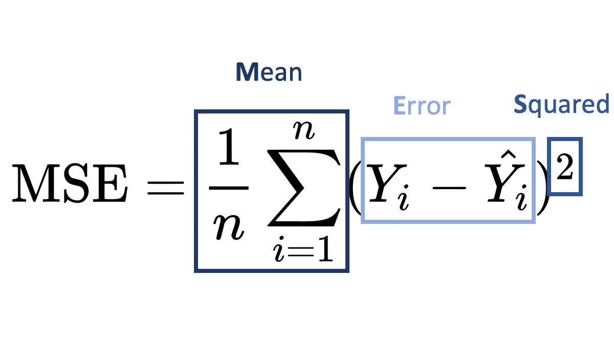
    MSLE (Mean Squared Logarithmic Error) and MSE (Mean Squared Error) are both loss functions that you can use in regression problems. But when should you use what metric?

    Mean Squared Error (MSE):

    It is useful when your target has a normal or normal-like distribution, as it is sensitive to outliers.

    An example is below –

    In this case using MSE as your loss function makes much more sense than MSLE.

    Mean Squared Logarithmic Error (MSLE):

    • MSLE measures the average squared logarithmic difference between the predicted and actual values.
    • MSLE treats smaller errors as less significant than larger ones due to the logarithmic transformation.
    • It is less sensitive to outliers than MSE since the logarithmic transformation compresses the error values.

    An example where you can use MSLE –

    Here if you use MSE then due to the exponential nature of the target, it will be sensitive to outliers and MSLE is a better metric, remember that MSLE cannot be used for optimisation, it is only an evaluation metric.

    In general, the choice between MSLE and MSE depends on the nature of the problem, the distribution of errors, and the desired behavior of the model. It’s often a good idea to experiment with both and evaluate their performance using appropriate evaluation metrics before finalizing the choice.

  • Numpy Argpartition – How it works?

    We all know that to find the maximum value index we can use argmax, but what if you want to find the top 3 or top 5 values. Then you can use argpartition.

    Let’s take an example array.

    x = [10,1,6,8,2,12,20,15,56,23]

    In this array, it’s very easy to find the maximum value index, it’s 8.

    But what if you want the top 3 or top 5, then you can use np.argmax.

    How it works is that it first sorts the array and then partitions the array on the kth element. All elements lower than the kth element will be behind it and larger ones will be after it.

    Let’s see with a few examples.

    idx = np.argpartition(x, kth=-3)
    print(idx)
    >>> [1 4 2 3 0 5 7 6 8 9]
    print([x[i] for i in idx ])
    >>> [1, 2, 6, 8, 10, 12, 15, 20, 56, 23]

    Here you can see that you get the top 3 indices as the last 3 values of the list, you can simply filter the values you can want by using idx[-3:].

    Similarly for the top 5 –

    idx = np.argpartition(x, kth=-5)
    print(idx[-5:])
    >>> [5 7 6 8 9]

    Hopefully, this post explains how you can use arg-partition to get the top k element indices. If you have any questions, feel free to ask in the comments or here on my Youtube Channel.

  • K-Nearest Neighbour Algorithm Explained

    KNN (K-Nearest Neighbours) is a supervised learning algorithm which uses the nearest neighbours to classify a new data point.

    The tricky part is selecting the optimal k for the model.

    sklearn.neighbors.KNeighborsClassifier(n_neighbors=5*weights='uniform'algorithm='auto'leaf_size=30p=2metric='minkowski'metric_params=Nonen_jobs=None)

    As you can see the weights by default is uniform and the n_neighbours is by default 5. Large values of k smooth things, but a very small value of k will be unreliable and could be affected by outliers.

    You can pick the optimal value of the k by tuning the hyperparameter using GridSearchCV.

    Then there is the value of p, which is by 2, meaning that it uses the euclidean distance, you can set it to 1 to use Manhattan distance. This is the distance it uses to chose the nearest points for classification.

    Let’s code this in python-

    from sklearn.neighbors import KNeighborsClassifier
    from sklearn.datasets import load_iris
    from sklearn.model_selection import GridSearchCV
    
    X, y = load_iris()['data'], load_iris()['target']
    
    #defining the search grid
    param_grid = {'n_neighbors': np.arange(3,10,1),
                 'p': [1,2,3]}
    
    grid_search = GridSearchCV(estimator=KNeighborsClassifier(), param_grid=param_grid, scoring='accuracy', cv = 3)
    
    grid_search.fit(X,y)
    
    print(grid_search.best_params_)
    >>> {'n_neighbors': 4, 'p': 2}
    print(grid_search.best_score_)
    >>>0.9866666666666667
    

    Hope this post cleared how you can use KNN in your machine learning problems, and if you want me to write about any ML topic, just drop a comment below.

  • ML Metrics | Top N Accuracy Explained

    This metric is usually used in multiclass classification problems.
    Each multiclass model gives a probability score for all the classes it is being trained on, but often you take the highest one, by using np.argmax but what if you took the top n classes and gave credit to the model if it got right in one of the n predictions.
    That is what is top n accuracy, it gives the model more chances to be right.

    Lets take an example.

    Suppose you built a model that predicts 3 classes and you want to find the top 2 accuracy of your model.
    Then you would pass the prediction array to the model and the true values and if the correct prediction is in the top 2 then you give it credit for being right.

    import numpy as np
    from sklearn.metrics import top_k_accuracy_score
    y_true = [0,1,1,2,2]
    y_pred = [[0.25, 0.2,0.3], #Here 0 is in the top 2
              [0.3, 0.35, 0.5], #Here 1 is in the top 2
              [0.2,0.4, 0.45], #Here 1 is in the top 2
              [0.5, 0.1, 0.2], #Here 2 is in the top 2
              [0.1, 0.4, 0.2]] #Here 2 is in the top 2
    top_k_accuracy_score(y_true, y_pred, k=2)
    

    It is 1.0, because the correct class was always in our top 2 prediction, actually, if you notice then it was always the second prediction of our model, so if we take regular accuracy or set the value k = 1 in top_k_accuracy_score(y_true, y_pred, k=2), the answer is 0.

    Hopefully, this explains what top N accuracy is, and if you want me to cover any ML topic, write in the comments below. Thanks for reading.

  • 5 Essential Boosting Parameters You Should Be Tuning

    Here are the 5 essential hyper-parameters that you should be always tuning when building any boosting model, whether you’re using XgBoost, LightGBM or even CatBoost.

    1. n_estimators – It is not the number of trees that the boosting algorithm will grow, but as the name suggests, the number of times gradient boosting will occur, so if you are using a tree-based boosting algorithm, then if you make this number 5, then each round of boosting fits a single tree to the negative gradient of some loss function.
    2. max_depth – The depth of each tree, pretty simple, the higher this number, the stronger each learner is in the model and the more your model can overfit. So pretty important to tune.
    3. learning_rate – Again a very important param, the higher it is the faster your algorithm will converge to the local minima, but too high and it might overshoot the minima, too low and it might never reach the minima.
    4. subsample – Sample of the training data to be used in each boosting round, if you use 0.5, then xgboost will randomly sample half your training data in each boosting iteration before growing the tree. Important if you want to control overfitting.
    5. colsample_bytree – Fraction of columns to use when growing a tree, again if set to 0.5, xgboost will randomly sample half of your features to grow the tree in each boosting round. Again very important to control overfitting.

    In another post I’ll be going over another 5 essential hyper-parameters that you should be tuning.

  • Pandas Essentials – Apply

    I often find people who are just starting out using pandas struggling to grasp when they should be using axis=0 and axis=1. While I go into a lot more detail with examples in the Youtube video above, you should keep this in mind.

    When you use axis=0, pandas only looks at the value being passed, but when you use axis=1, by default it assumes a pandas Series being passed, so it looks for the index. So when you write a function which references multiple columns and use apply, use axis=1 and remember that it considers each row as a pandas Series, with the column names in the index.