Suppose you want to calculate aggregated count features and add them to your data frame as a feature. What you would typically do is, create a grouped data frame and then do a join. What if you can do all that in just one single line of code. Here you can use the transform functionality in pandas.
import numpy as np
import pandas as pd
import seaborn as sns
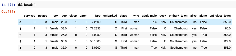
df = sns.load_dataset('titanic')
df.head()
Using df['cnt_class_town'] = df.groupby(['class', 'embark_town']).transform('size') we can directly get our desired feature in the data frame.
Again, if you want to create any sort of binned features based on the quantiles, usually first you would create a function and then use pandas apply to add that bucket to your data. Here again, you can directly use qcut functionality from pandas, pandas.qcut(x, q, labels=None, retbins=False, precision=3, duplicates='raise') to create the buckets in just one line of code.
Let’s take an example where we want to bin the age column into 4 categories, we can do so by running this one line of code –
We know that calculating the correlation between numerical variables is very easy, all you have to do is call df.corr().
But how do you calculate the correlation between categorical variables?
If you have two categorical variables then the strength of the relationship can be found by using Chi-Squared Test for independence.
The Chi-square test finds the probability of a Null hypothesis (H0).
Assumption(H0): The two columns are not correlated. H1: The two columns are correlated. Result of Chi-Sq Test: The Probability of H0 being True
We will be using the titanic dataset to calculate the chi-squared test for independence on a couple of categorical variables.
import numpy as np
import pandas as pd
import seaborn as sns
from matplotlib import pyplot as plt
df = sns.load_dataset('titanic')
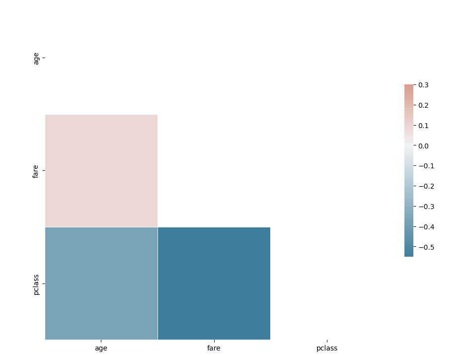
corr = df[['age', 'fare', 'pclass']].corr()
# Generate a mask for the upper triangle
mask = np.triu(np.ones_like(corr, dtype=bool))
# Set up the matplotlib figure
f, ax = plt.subplots(figsize=(11, 9))
# Generate a custom diverging colormap
cmap = sns.diverging_palette(230, 20, as_cmap=True)
# Draw the heatmap with the mask and correct aspect ratio
sns.heatmap(corr, mask=mask, cmap=cmap, vmax=.3, center=0,
square=True, linewidths=.5, cbar_kws={"shrink": .5})
Pretty easy to calculate the correlation among numerical variables.
Lets first calculate first whether the class of the passenger and whether or not they survive have a correlation.
# importing the required function
from scipy.stats import chi2_contingency
cross_tab=pd.crosstab(index=df['class'],columns=df['survived'])
print(cross_tab)
chi_sq_result = chi2_contingency(cross_tab,)
p, x = chi_sq_result[1], "reject" if chi_sq_result[1] < 0.05 else "accept"

print(f"The p-value is {chi_sq_result[1]} and hence we {x} the null Hpothesis with {chi_sq_result[2]} degrees of freedom")
The p-value is 4.549251711298793e-23 and hence we reject the null Hpothesis with 2 degrees of freedom
Similarly, we can calculate whether two categorical variables are correlated amongst other variables as well.
Hopefully, this clears up how you can calculate whether two categorical variables are correlated or not in python. In case you have any questions please feel free to ask them in the comments.
In Part 1 of this series, we covered how you can use lag features and simple linear regression models to do time series forecasting, but that is very simple and you cannot capture trends using that model which is non-linear.
So we will be discussing different types of moving averages you can calculate in python and how they are helpful.
Simple Moving Average
# Loading Libraries
import numpy as np
import pandas as pd
import seaborn as sns
sns.set_theme()
#Using the available dowjones data in seaborn
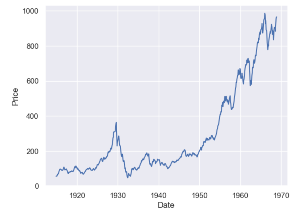
dowjones = sns.load_dataset("dowjones")
dowjones.head()
sns.lineplot(data=dowjones, x="Date", y="Price")
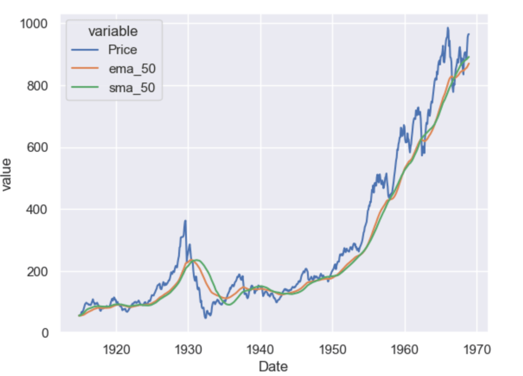
A simple moving average (SMA) calculates the average of a selected range of values, by the number of periods in that range. The most typical moving averages are 30-day, 50-day, 100-day and 365 day moving averages. Moving averages are nice cause they can determine trends while ignoring short-term fluctuations. One can calculate the sma by simply using
As you can see the higher the value of the window, the lesser it is affected by short-term fluctuations and it captures long-term trends in the data. Simple Moving Averages are often used by traders in the stock market for technical analysis.
Exponential Moving Average
Simple moving averages are nice, but they give equal weightage to each of the data points, what if you wanted an average that will give higher weight to more recent points and lesser to points in the past. In that case, what you want is to compute the exponential moving average (EMA).
As you can see the ema_50 follows the Price chart more closely than the sma_50 and is more sensitive to the recent data points.
Which moving average you should use as a feature of your forecasting model is a question mostly dependent on the use case. However, you will often use some kind of moving average as a feature or to visualise long-term or short-term trends in your data.
In Part 3 we explore trends and seasonality and how can you identify them in your data.
In this series of posts, I’ll be covering how to approach time series forecasting in python in detail. We will start with the basics and build on top of it. All posts will contain a practice example attached as a GitHub Gist. You can either read the post or watch the explainer Youtube video below.
# Loading Libraries
import numpy as np
import pandas as pd
import seaborn as sns
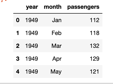
We will be using a simple linear regression to predict the outcome of the number of flights in the month of May. The data is taken from seaborn datasets.
As you can see we’ve the year, the month and the number of passengers, as a dummy example we will focus on the number of passengers in the month of May, below is the plot of year vs passengers.
We can clearly see a pattern here and can build a simple linear regression model to predict the number of passengers in the month of May in future years. The model will be like y = slope * feature + intercept. The feature, in this case, will be the number of passengers but shifted by 1 year. Meaning the number of passengers in the year 1949 will be the feature for the year 1950 and so on.
We can see that the p-value of the feature is significant, the intercept is not so significant, and the R-squared value is 0.97 which is very good. Of course, this is a dummy example so the values will be good.
df['prediction'] = df['lag_1']*m + b
sns.lineplot(x='year', y='value', hue='variable',
             data=pd.melt(df, ['year']))
So today I was participating in this Kaggle competition and the data had too many categorical variables. One way to build a model with too many categorical variables is to use a model like Catboost and let it deal with encoding categorical variables. But I wanted to ensemble my results with an Xgboost model, so I had to encode them. Using the weight of evidence encoding, I got a solution which was a top 10 solution when submitted. I have made the notebook public, you can go here and see it.
So what is weight of evidence ?
To put it simply –
I’ve gone through an example explaining the weight of evidence in the youtube video below.
One often thinks that you can use deep learning for classification problems like text or image classification, or for similar tasks like segmentation, language models etc. But you can also do simple linear regression with deep learning libraries. I’ve also attached the GitHub Gist in case you want to explore the working notebook.
In this post I’ll go over the model, it’s explanation on how can you do linear regression with keras.
In Keras, it can be implemented using the Sequential model and the Dense layer. Here’s an example of how to implement linear regression with Keras:
First we take a toy regression problem from scikit-learn datasets.
from sklearn.datasets import load_diabetes
from sklearn.model_selection import train_test_split

X,y = load_diabetes(return_X_y=True)

X_train, X_test, y_train, y_test = train_test_split(X,y, train_size=0.8)
Now we will need to define the model using Keras. That is actually very simple, you just have to take one sequential model with a Dense layer. The activation for this layer will be linear as we’re building a linear model and the loss will be mean squared error.
import numpy as np
from keras.models import Sequential
from keras.layers import Dense

# define the model
model = Sequential()
model.add(Dense(units=1, activation='linear'))
# compile the model
model.compile(optimizer='sgd', loss='mean_squared_error', metrics = ['mae'])

#fit the model
model.fit(x=X_train, y=y_train, validation_data=(X_test,y_test),
          epochs=100, batch_size=128)
Thats then all that is left is to call model.predict(X_test).
In this post, we will go over the complete decision tree theory and also build a very basic decision tree using information gain from scratch.
The below jupyter notebook as a Github Gist shows all the explanations and steps, including how to calculate Gini, Information gain and building a decision tree using the information gain you calculate.
You can also watch the video explainer here on youtube.
Random projection is another dimensionality reduction algorithm like PCA, as the name suggests, the basic idea behind Random Projection is to map the original high-dimensional data onto a lower-dimensional space while preserving as much of the pairwise distances between the data points as possible. This is done by generating a random matrix of size (n x k) where n is the dimensionality of the original data and k is the desired dimensionality of the reduced data.
If we have a matrix M of dimension and another matrix R of dimension whose columns are representing random directions, the random projection of M is then calculated as
The idea behind random projection is similar to PCA, but in PCA we first compute the eigenvalues, here we project the vector on random directions without any complex computations.
The random matrix used for the projection can be generated in a variety of ways. One popular method is the Johnson-Lindenstrauss lemma, which states that the pairwise distances between the points in the original space can be approximately preserved if the dimensionality of the lower-dimensional space is chosen to be logarithmic in the number of data points. Another popular method is the use of random gaussian matrix.
The Gaussian random projection reduces the dimensionality by projecting the original input space on a randomly generated matrix where components are drawn from the following distribution .
Why use Random Projection in place of PCA ?
Random Projection is often used in large-scale data analysis and machine learning applications where computational resources are limited and the dimensionality of the data is too high. In such cases, calculating PCA is often too time-consuming and computationally expensive. Additionally, Random Projection is less sensitive to the presence of noise and outliers in the data compared to PCA.
Sometimes, coding questions are also part of data science interviews, so here is the solution to LeetCode #11 – the container with the most water problem.
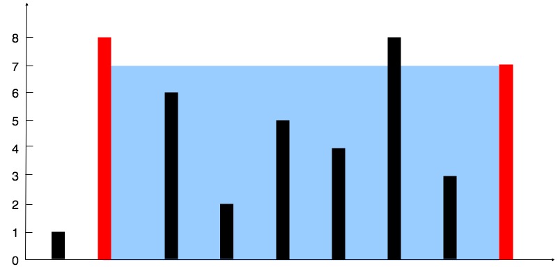
The problem is very straightforward, you’re given a list with n integers, each representing the height of a tower, you’ve to find the maximum area that can be formed with these heights and the x-axis represents the index distance between the integers with a twist that since it represents a block containing water, you’ve to take the min of the two heights as the water has to contained within the towers.
For example, if the list of given heights is h = [1,1,4,5,10,1], the maximum area that can be formed will be 8. It will be between the tower with heights 4 and 10, with an index distance of 2. So the area will be min(4,10)*2 = 8.
Coming to the solution, the easiest solution will be to compare each combination of two tower heights, and return the maximum area that can be formed. This will have a time complexity of
def maxArea(height: List[int]) -> int:
        max_vol = 0
        for i in range(len(height)):
            for j in range(1,len(height)):
                if j<=i:
                    continue
                else:
                    vol = min(height[i], height[j])*(j-i)
                    max_vol = max(max_vol, vol)
        return max_vol
Although the above solution will pass the sample test cases, it will eventually return Time Limit Exceeded as it is a very brute force solution, as it compares almost every possible combination. You can be a bit more clever in your approach and solve this problem in time complexity.
The trick is using pointers, one for left and one for right, starting with the largest width and then storing the max area. Move the left pointer right if you encounter a higher tower in the left otherwise move the right pointer towards the left, and repeat till both pointers meet. In this way, you’ve traversed the list only once.
def maxArea(height: List[int]) -> int:
        l,r = 0,len(height) - 1
        max_vol = -1
        while l < r:
            #Calculating the shorter height of the two
            shorter_height = min(height[l], height[r])
            width = r-l
            vol = shorter_height * width
            max_vol = max(vol, max_vol)
            if height[l] < height[r]:
                l+=1
            else:
                r-=1
        return max_vol
Taking an example, if input is [1,4,5,7,4,1], then.
Step
l
r
width
min height
area
max area
1
0
5
5
1
5
5
2
0
4
4
1
4
5
3
1
4
3
4
12
12
4
1
3
2
4
8
12
5
2
3
1
5
5
12
The loop will exit after step 5 as in step 6 l = r = 3, and we get the max area as 12.
While the questions that you may be asked in a data science interview can vary a lot depending on the job description and the skillsets the organisation is looking for, there are a few questions that are often asked and as a candidate, you should know the answer to these.
Here in this post I’ll try to cover 10 such questions that you should know –
1. What is Bias-Variance Trade-off?
Bias in very simple terms is the error of your ML model. Variance is the difference in the evaluation metric in the train set and the test set that your model achieves. With any machine learning model, you try to reduce both bias and variance. The bias-variance trade-off is as you reduce bias, variance usually increases. So you try to select the ML model which has the lowest bias and variance. The below diagram should explain bias and variance.
2. In multiple linear regression if you keep adding dependent variables, the coefficient of determination (R-squared value) keeps going up, how do you then measure whether the model is improving or not?
In case of multiple linear regression, in addition to the you also calculate the adjusted r2, , which adjusts for the number of variables in the model and penalizes models with an excessive number of variables.
You should stop adding dependent variables when the adjusted r2 values starts to worsen
3. How does Random Forest reduce variance?
The main idea behind the Random Forest algorithm is to use low-bias decision trees and aggregate their results to reduce variance. Since each tree is grown from a bagged sample and also the features are bagged, meaning that each tree is grown from a different subset of features, thus the trees are not correlated and hence their combined results lead to lower variance than a single decision tree with low bias and high variance.
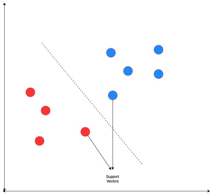
4. What are the support vectors in support vector machine (SVM)?
The support vectors are the data points that are used to define the decision boundary, or hyperplane, in an SVM. They are the key data points that determine the position of the decision boundary, and any change in these support vectors will result in a change in the decision boundary.
5. What is cross-validation and how is it used to evaluate a model’s performance?
Cross-validation involves dividing the available data into two sets: a training set and a validation set. The model is trained on the training set, and its performance is evaluated on the validation set. This process is repeated multiple times with different partitions of the data, and the performance measure is averaged across all iterations. This gives a more robust estimation of the model’s performance than a single train test split can do.
There are different types of cross-validation methods like k-fold cross-validation, in which the data is divided into k-folds, and the model is trained on k-1 folds and tested on the remaining fold. This process is repeated k times, and the performance measure is averaged across all iterations. Another one is Leave one out Cross-validation(LOOCV), in this method we use n-1 observations for training and the last one for testing. There is also a time-series cross-validation where the model is trained till time t and tested for a time after t. The window of training time keeps expanding after each iteration, it is also called expanding window cross-validation for time series.
I’ll be posting more Data Science questions on the blog so keep following for updates.


 and another matrix R of dimension
  whose columns are representing random directions, the random projection of M is then calculated as
 .
.

 time complexity.
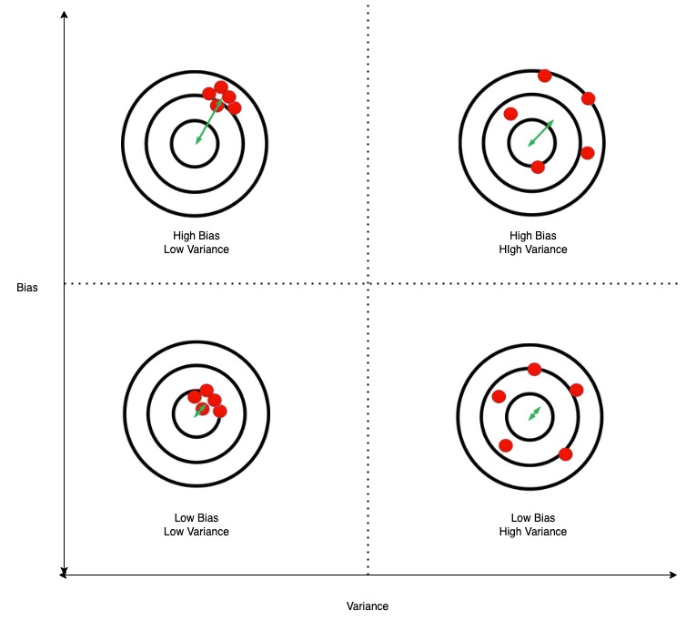
 you also calculate the adjusted r2,
  , which adjusts for the number of variables in the model and penalizes models with an excessive number of variables.