MSLE (Mean Squared Logarithmic Error) and MSE (Mean Squared Error) are both loss functions that you can use in regression problems. But when should you use what metric?
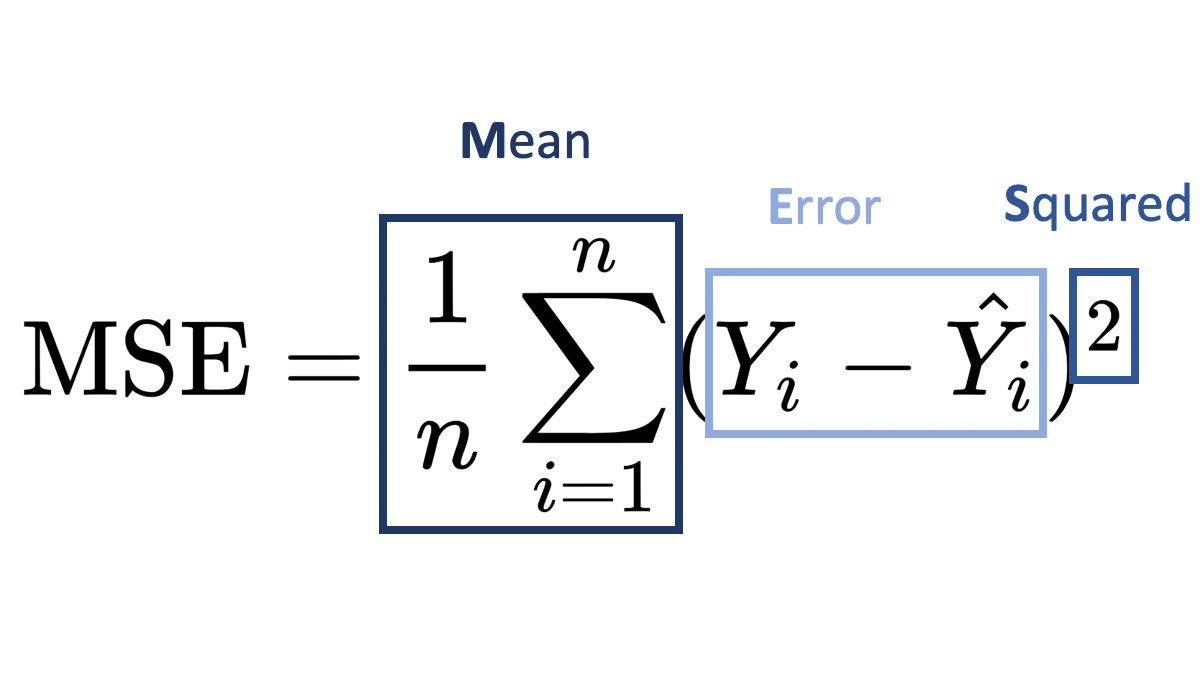
Mean Squared Error (MSE):
It is useful when your target has a normal or normal-like distribution, as it is sensitive to outliers.
An example is below –
In this case using MSE as your loss function makes much more sense than MSLE.
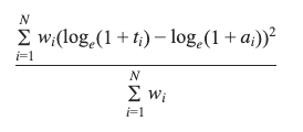
Mean Squared Logarithmic Error (MSLE):
MSLE measures the average squared logarithmic difference between the predicted and actual values.
MSLE treats smaller errors as less significant than larger ones due to the logarithmic transformation.
It is less sensitive to outliers than MSE since the logarithmic transformation compresses the error values.
An example where you can use MSLE –
Here if you use MSE then due to the exponential nature of the target, it will be sensitive to outliers and MSLE is a better metric, remember that MSLE cannot be used for optimisation, it is only an evaluation metric.
In general, the choice between MSLE and MSE depends on the nature of the problem, the distribution of errors, and the desired behavior of the model. It’s often a good idea to experiment with both and evaluate their performance using appropriate evaluation metrics before finalizing the choice.
We know that calculating the correlation between numerical variables is very easy, all you have to do is call df.corr().
But how do you calculate the correlation between categorical variables?
If you have two categorical variables then the strength of the relationship can be found by using Chi-Squared Test for independence.
The Chi-square test finds the probability of a Null hypothesis (H0).
Assumption(H0): The two columns are not correlated. H1: The two columns are correlated. Result of Chi-Sq Test: The Probability of H0 being True
We will be using the titanic dataset to calculate the chi-squared test for independence on a couple of categorical variables.
import numpy as np
import pandas as pd
import seaborn as sns
from matplotlib import pyplot as plt
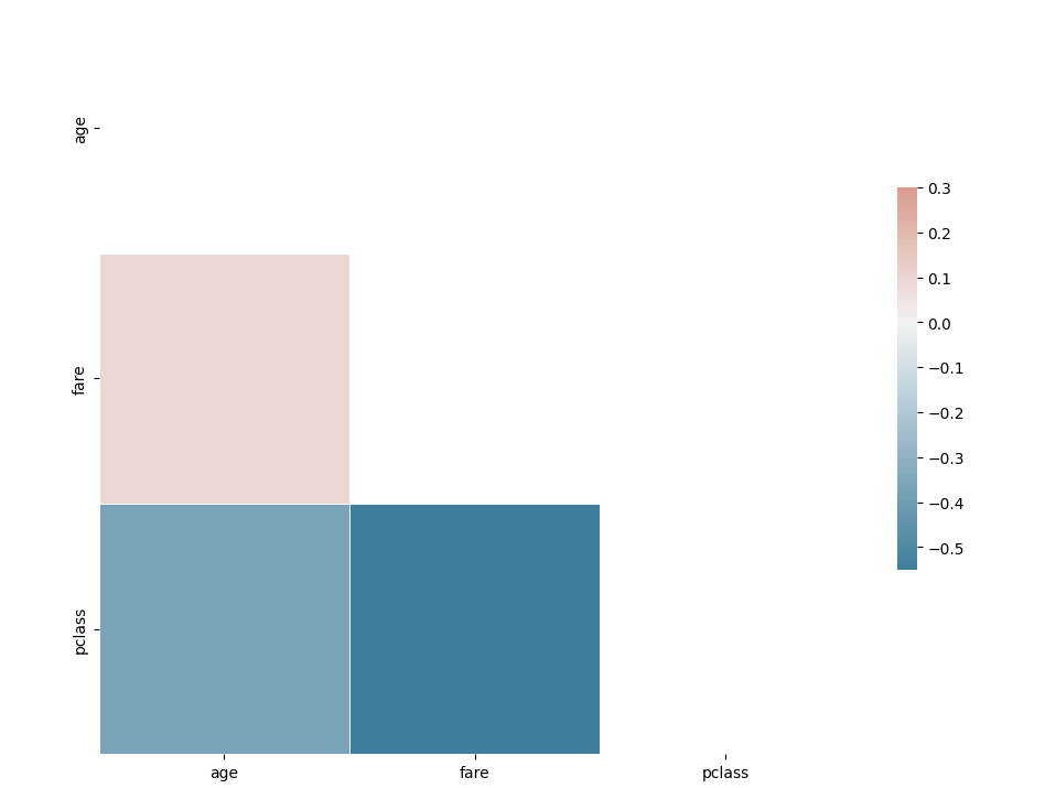
df = sns.load_dataset('titanic')
corr = df[['age', 'fare', 'pclass']].corr()
# Generate a mask for the upper triangle
mask = np.triu(np.ones_like(corr, dtype=bool))
# Set up the matplotlib figure
f, ax = plt.subplots(figsize=(11, 9))
# Generate a custom diverging colormap
cmap = sns.diverging_palette(230, 20, as_cmap=True)
# Draw the heatmap with the mask and correct aspect ratio
sns.heatmap(corr, mask=mask, cmap=cmap, vmax=.3, center=0,
square=True, linewidths=.5, cbar_kws={"shrink": .5})
Pretty easy to calculate the correlation among numerical variables.
Lets first calculate first whether the class of the passenger and whether or not they survive have a correlation.
# importing the required function
from scipy.stats import chi2_contingency
cross_tab=pd.crosstab(index=df['class'],columns=df['survived'])
print(cross_tab)
chi_sq_result = chi2_contingency(cross_tab,)
p, x = chi_sq_result[1], "reject" if chi_sq_result[1] < 0.05 else "accept"

print(f"The p-value is {chi_sq_result[1]} and hence we {x} the null Hpothesis with {chi_sq_result[2]} degrees of freedom")
The p-value is 4.549251711298793e-23 and hence we reject the null Hpothesis with 2 degrees of freedom
Similarly, we can calculate whether two categorical variables are correlated amongst other variables as well.
Hopefully, this clears up how you can calculate whether two categorical variables are correlated or not in python. In case you have any questions please feel free to ask them in the comments.
In this series of posts, I’ll be covering how to approach time series forecasting in python in detail. We will start with the basics and build on top of it. All posts will contain a practice example attached as a GitHub Gist. You can either read the post or watch the explainer Youtube video below.
# Loading Libraries
import numpy as np
import pandas as pd
import seaborn as sns
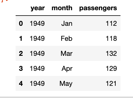
We will be using a simple linear regression to predict the outcome of the number of flights in the month of May. The data is taken from seaborn datasets.
As you can see we’ve the year, the month and the number of passengers, as a dummy example we will focus on the number of passengers in the month of May, below is the plot of year vs passengers.
We can clearly see a pattern here and can build a simple linear regression model to predict the number of passengers in the month of May in future years. The model will be like y = slope * feature + intercept. The feature, in this case, will be the number of passengers but shifted by 1 year. Meaning the number of passengers in the year 1949 will be the feature for the year 1950 and so on.
We can see that the p-value of the feature is significant, the intercept is not so significant, and the R-squared value is 0.97 which is very good. Of course, this is a dummy example so the values will be good.
df['prediction'] = df['lag_1']*m + b
sns.lineplot(x='year', y='value', hue='variable',
             data=pd.melt(df, ['year']))
One often thinks that you can use deep learning for classification problems like text or image classification, or for similar tasks like segmentation, language models etc. But you can also do simple linear regression with deep learning libraries. I’ve also attached the GitHub Gist in case you want to explore the working notebook.
In this post I’ll go over the model, it’s explanation on how can you do linear regression with keras.
In Keras, it can be implemented using the Sequential model and the Dense layer. Here’s an example of how to implement linear regression with Keras:
First we take a toy regression problem from scikit-learn datasets.
from sklearn.datasets import load_diabetes
from sklearn.model_selection import train_test_split

X,y = load_diabetes(return_X_y=True)

X_train, X_test, y_train, y_test = train_test_split(X,y, train_size=0.8)
Now we will need to define the model using Keras. That is actually very simple, you just have to take one sequential model with a Dense layer. The activation for this layer will be linear as we’re building a linear model and the loss will be mean squared error.
import numpy as np
from keras.models import Sequential
from keras.layers import Dense

# define the model
model = Sequential()
model.add(Dense(units=1, activation='linear'))
# compile the model
model.compile(optimizer='sgd', loss='mean_squared_error', metrics = ['mae'])

#fit the model
model.fit(x=X_train, y=y_train, validation_data=(X_test,y_test),
          epochs=100, batch_size=128)
Thats then all that is left is to call model.predict(X_test).
While the questions that you may be asked in a data science interview can vary a lot depending on the job description and the skillsets the organisation is looking for, there are a few questions that are often asked and as a candidate, you should know the answer to these.
Here in this post I’ll try to cover 10 such questions that you should know –
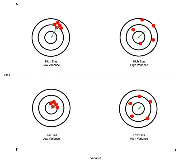
1. What is Bias-Variance Trade-off?
Bias in very simple terms is the error of your ML model. Variance is the difference in the evaluation metric in the train set and the test set that your model achieves. With any machine learning model, you try to reduce both bias and variance. The bias-variance trade-off is as you reduce bias, variance usually increases. So you try to select the ML model which has the lowest bias and variance. The below diagram should explain bias and variance.
2. In multiple linear regression if you keep adding dependent variables, the coefficient of determination (R-squared value) keeps going up, how do you then measure whether the model is improving or not?
In case of multiple linear regression, in addition to the you also calculate the adjusted r2, , which adjusts for the number of variables in the model and penalizes models with an excessive number of variables.
You should stop adding dependent variables when the adjusted r2 values starts to worsen
3. How does Random Forest reduce variance?
The main idea behind the Random Forest algorithm is to use low-bias decision trees and aggregate their results to reduce variance. Since each tree is grown from a bagged sample and also the features are bagged, meaning that each tree is grown from a different subset of features, thus the trees are not correlated and hence their combined results lead to lower variance than a single decision tree with low bias and high variance.
4. What are the support vectors in support vector machine (SVM)?
The support vectors are the data points that are used to define the decision boundary, or hyperplane, in an SVM. They are the key data points that determine the position of the decision boundary, and any change in these support vectors will result in a change in the decision boundary.
5. What is cross-validation and how is it used to evaluate a model’s performance?
Cross-validation involves dividing the available data into two sets: a training set and a validation set. The model is trained on the training set, and its performance is evaluated on the validation set. This process is repeated multiple times with different partitions of the data, and the performance measure is averaged across all iterations. This gives a more robust estimation of the model’s performance than a single train test split can do.
There are different types of cross-validation methods like k-fold cross-validation, in which the data is divided into k-folds, and the model is trained on k-1 folds and tested on the remaining fold. This process is repeated k times, and the performance measure is averaged across all iterations. Another one is Leave one out Cross-validation(LOOCV), in this method we use n-1 observations for training and the last one for testing. There is also a time-series cross-validation where the model is trained till time t and tested for a time after t. The window of training time keeps expanding after each iteration, it is also called expanding window cross-validation for time series.
I’ll be posting more Data Science questions on the blog so keep following for updates.
I was going through Kaggle competitions when this competition caught my eye, especially the evaluation metric for it. Now the usual metrics for forecasting or regression problems are either or , but sMAPE is different.
SMAPE (Symmetric Mean Absolute Percentage Error) is a metric that is used to evaluate the accuracy of a forecast model. It is calculated as the average of the absolute percentage differences between the forecasted and actual values, with the percentage computed using the actual value as the base. Mathematically, it can be expressed as:
So when to use which metric ?
RMSE – When you want to penalize large outlier errors in your prediction model, RMSE is the metric of choice as it penalizes large errors more than smaller ones.
MAPE – All errors have to be treated equally, so in those cases MAPE makes sense to use
sMAPE – is typically used when the forecasted values and the actual values are both positive, and when the forecasts and actuals are of similar magnitudes. It is symmetric in that it treats over-forecasting and under-forecasting the same.
It is important to note that in both MAPE and sMAPE, values of 0 are not allowed for both actual and forecast values as it would result in division by zero error.
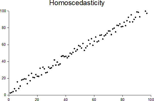
Once your linear regression model is trained, you should always plot your residuals (y – ŷ) whether the errors are homoscedastic or heteroscedastic. What do we mean by these terms? It means that there should not be any pattern in residuals and they should be uniformly distributed, or in other words, there should not be any variance in the residuals. Homoscedasticity is one of the assumptions of linear regression, so it is often important to check for it.
source: Wikipedia
source: Wikipedia
In the above figures, you can clearly see that the residuals have a clear pattern in the heteroscedastic image. In that scenario, you cannot rely on the regression analysis.
How to test for heteroscedasticity?
There are many ways to test for heteroscedasticity, I’ll list a. few ways here –
Visual Test – Just look at the residual plot and you’ll often see whether the residuals have any variance or not, not very accurate but often works.
Bartlett test
Breusch Pagan test
Goldfeld Quandt test
Glesjer test
Test based on Spearman’s rank correlation coefficient
White test
Ramsey test
Harvey Phillips test
Szroeter test
Peak test (nonparametric) test
All these tests in one way or another try to reject the null hypothesis H0 : variance is constant and the alternative hypothesis is that Ha : variance is not constant. You can go into detail about the tests here.
Variance Inflation Factor (VIF) determines the multicollinearity amongst the independent variables (predictors). Multicollinearity is when there is a high correlation between your predictor variables, usually 0.8 or higher. This can adversely affect your regression analysis.
How is it calculated?
VIF of a predictor variable is calculated by regressing it against all other predictor variables. This gives the R2 value which can be plugged into this formula
This will give the VIF value of a predictor.
VIF = 1, not correlated
VIF < 5, slightly correlated
VIF > 5, highly correlated
These values are just guidelines and how high acceptable VIF values are depends on the problem statement.
If you don’t want to use VIF and have very few predictor variables, one can plot a correlation matrix and remove the highly correlated variables.
You might also wonder why do we calculate the p-value of predictor variables in Linear regression. Find out why here.
Ever wondered why we look for p-value less than 0.05 for the coefficients when looking at the linear regression results.
Let’s quickly recap the basics of linear regression. In Linear Regression we try to estimate a best fit line for given data points. In case we have only one predictor variable and a target the linear equation will look something like
Y = A + Bx
Here A being the intercept and B being the slope or coefficient.
The null hypothesis for linear regression is that B=0 and the alternate hypothesis is that B != 0.
This is the reason why we look for p-value < 0.05 to reject the null hypothesis and establish that there exists a relationship between the target and the predictor variable.


 you also calculate the adjusted r2,
  , which adjusts for the number of variables in the model and penalizes models with an excessive number of variables.
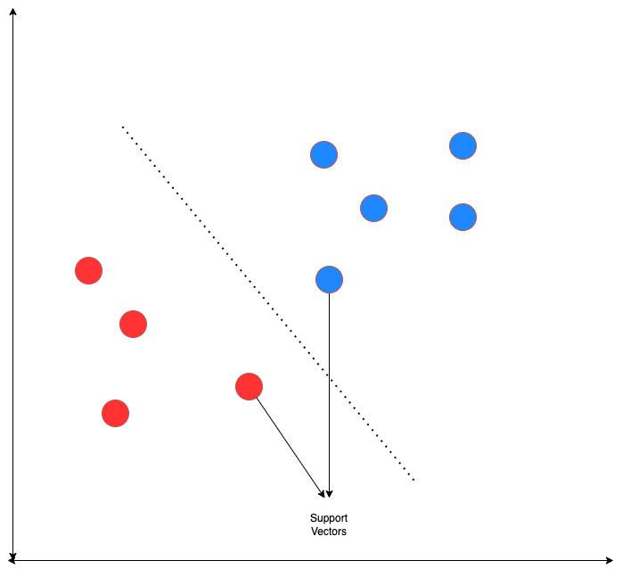
 or
or  , but sMAPE is different.