Tag: Machine Learning

Q-Learning in Python: Reinforcement Learning on Frozen Lake
Ever seen an AI agent go from stumbling around cluelessly to mastering its environment, making perfect moves every single time? In this blog post, we’ll explore how to train an agent to do just that, transforming random, chaotic actions into smooth, optimal choices. We’ll dive into the fascinating world of Q-learning and discover how it empowers AI agents to learn and adapt. In case you want to follow along, here is the link to the collab notebook.

What Is Q-Learning ?

Q-learning is a type of reinforcement learning where an agent learns to make optimal decisions by interacting with its environment. The agent explores its surroundings, tries different actions, and observes the outcomes. It uses a Q-table to store Q-values, which represent the expected reward for taking a specific action in a given state. Over time, the agent updates its Q-values based on its experiences, gradually learning the best actions to take in each situation.

source: HuggingFace

The Q-value update formula takes in our former estimate of the Q-value and then adds the temporal difference error, which is crucial for correctly adjusting our predictions based on new information. We multiply this value by a learning rate to take small, manageable steps, akin to the incremental updates we see in machine learning algorithms, allowing for gradual refinement of our estimates. The Temporal Difference Error is particularly significant as it comprises not just the immediate reward received from a given action, but also includes the discounted estimate of the optimal Q-value in the next state that our selected action will lead us into; this next step’s predicted value is critical as it influences our future decisions. This entire process is essential for the learning agent to adapt effectively to its environment, correction of biases in the initial Q-value estimates, and thus improving the overall decision-making strategy. By subtracting this former estimate of the Q-value from the combined factors, we arrive at a refined estimate that enhances the agent’s ability to predict and maximize long-term rewards in a dynamic setting.

The Frozen Lake Environment

Enough of theory, now it’s time to train our agent on the Frozen Lake Environment. Imagine a frozen lake with slippery patches. Our agent’s goal is to navigate across the lake without falling into any holes. The agent can move up, down, left, or right, but the slippery surface makes its actions unpredictable. This simple environment provides a great starting point for understanding Q-learning. We will go over the training on the non-slipper environment. To see how the agent performs in the slippery environment, you can see the YouTube video for this.

The first thing we will have to do is to initialize the environment.
```
# Importing libraries
import gymnasium as gym
import numpy as np
from matplotlib import pyplot as plt

np.set_printoptions(precision=3)

env = gym.make('FrozenLake-v1', desc=None, map_name="4x4", is_slippery=False, render_mode="rgb_array")
print(f"There are {env.action_space.n} possible actions")
print(f"There are {env.observation_space.n} states")
>>>There are 4 possible actions
>>>There are 16 states
```
We can see that our world is 4×4 in size and thus has 16 possible states and there are 4 possible actions – up, down, left and right. We can take a look at the world.

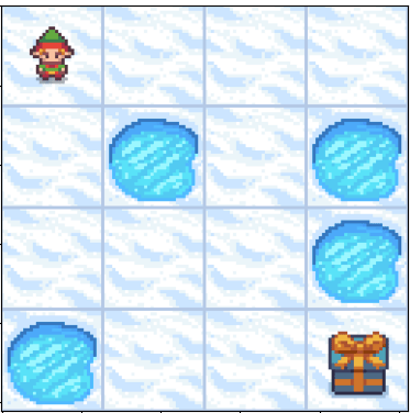
The goal of our agent is to reach the prize at the bottom-right. We can clearly see that it can do so by either going right->right->down->down->down->right or by following down->down->right->right->down->right. But how do we train the agent to come up with either of these path on its own.

We do so by initially letting the agent explore the environment randomly, trying different actions to see what happens, without any predefined strategy guiding its decisions. This phase of exploration is crucial, as it allows the agent to gather diverse experiences and build a foundational understanding of the environment’s dynamics. As it gains experience over time, it starts exploiting its learned knowledge, choosing actions with higher Q-values that have been identified as beneficial through previous trials. This shift from exploration to exploitation represents a significant turning point in the agent’s learning process, where it leverages its accumulated data to make more informed decisions. Throughout its journey, the agent balances exploration and exploitation to ensure it both discovers new strategies and utilizes its existing knowledge effectively. By continuously adjusting this balance, the agent enhances its performance, ultimately leading to more efficient learning and improved decision-making capabilities in complex scenarios.

To do so let’s establish some helper functions first –
```
def get_action(epsilon, state, q_table):
    if np.random.rand() < epsilon:
        return np.random.randint(0, env.action_space.n)
    else:
        return np.argmax(q_table[state])

def get_td_error(state, next_state, action, reward, q_table):
    former_q_est = q_table[state,action]
    td_target = reward+ gamma*np.max(q_table[next_state])
    td_error = td_target - former_q_est
    return td_error

# As seen, we first define the Q-table and during the training epochs we update this value. 
q_table = np.zeros((env.observation_space.n, env.action_space.n))
```
We created two functions, The first function, get_action, determines the action based on epsilon, which controls the randomness of our actions.. Initially during training we keep the epsilon very high and lower it as the agent learns. The second function, get_td_error, calculates the temporal difference error after each step. We also created our q-table which is a combination n_states x n_actions= 16×4.

We also have to establish training hyper-parameters.
```
num_epochs = 1000
gamma = 0.99
lr = 0.1
decay_rate=0.99
epsilon = 1
```
During training, in each epoch we update our q-table after each action. The epoch is done if we either fall into the hole or get to the prize. After the episode is done we decay the epsilon a bit and repeat the process again. After the training is done our q-table should have converged to optimal q-values for each state-action pair.
```
for i in range(num_epochs):
    state, _ = env.reset()
    done = False
    while not done:
        action = get_action(epsilon, state, q_table)
        next_state, reward, done, _, _ = env.step(action)
        td_error = get_td_error(state, next_state, action, reward, q_table)
        q_table[state, action] = q_table[state, action] + lr*td_error
        state = next_state
    epsilon*=decay_rate
```
Now that we’ve trained our agent, let’s see how it’s action looks like. The code for creating the animation is in the collab notebook.

We can see that it always now follows the optimal path.

Conclusion

Q-learning is a powerful technique for training AI agents to make optimal decisions. By interacting with their environment and learning from their experiences, agents can master even complex tasks. As we’ve seen, the environment plays a crucial role in shaping the agent’s behavior.

However, in complex environments with a vast number of states, traditional Q-learning becomes impractical. That’s where deep Q-learning comes in. By using deep neural networks, we can approximate Q-values without relying on an enormous Q-table. Stay tuned for our next blog post, where we’ll explore the intricacies of deep Q-learning.
November 9, 2024

From Certain to Uncertain | Stochastic Bellman Equation Made Easy

In the video below we will go over how to calculate value for a state when the actions are probabilistic.

If you wondered how do I get the values for all states, here is the code snippet for it.

import numpy as np
import matplotlib.pyplot as plt
from typing import List, Tuple

class StochasticGridWorld:
    def __init__(self, size: int = 3, gamma: float = 0.9):
        self.size = size
        self.gamma = gamma
        # Initialize states
        self.values = np.zeros((size, size))
        self.values[0, 2] = -1  # Cat
        self.values[2, 2] = 1   # Cheese
        
        # Track value history for convergence visualization
        self.value_history = {(i, j): [] for i in range(size) for j in range(size)}
        
        # Movement probabilities
        self.p_intended = 0.5  # Probability of moving in intended direction
        self.p_random = 0.5 / 4  # Split remaining probability among all directions
        
    def get_next_state(self, current_state: Tuple[int, int], 
                       action: Tuple[int, int]) -> Tuple[int, int]:
        """Calculate next state given current state and action"""
        next_i = current_state[0] + action[0]
        next_j = current_state[1] + action[1]
        
        # Check if next state is within grid
        if 0 <= next_i < self.size and 0 <= next_j < self.size:
            return (next_i, next_j)
        return current_state
    
    def get_possible_actions(self) -> List[Tuple[int, int]]:
        """Return all possible actions as (dx, dy)"""
        return [(0, 1), (0, -1), (1, 0), (-1, 0)]  # Right, Left, Down, Up
    
    def calculate_state_value(self, state: Tuple[int, int]) -> float:
        """Calculate value for a given state considering all actions"""
        if state == (0, 2) or state == (2, 2):  # Terminal states
            return self.values[state]
        
        max_value = float('-inf')
        actions = self.get_possible_actions()
        
        for action in actions:
            value = 0 # We know this as the immediate reward is 0
            # Intended movement
            next_state = self.get_next_state(state, action)
            value += self.p_intended * self.values[next_state]
            
            # Random movements
            for random_action in actions:
                random_next_state = self.get_next_state(state, random_action)
                value += self.p_random * self.values[random_next_state]
            
            value = self.gamma * value  # Apply discount factor
            max_value = max(max_value, value)
            
        return max_value
    
    def value_iteration(self, num_iterations: int = 100, 
                       threshold: float = 1e-4) -> np.ndarray:
        """Perform value iteration and store history"""
        for iteration in range(num_iterations):
            delta = 0
            new_values = np.copy(self.values)
            
            for i in range(self.size):
                for j in range(self.size):
                    if (i, j) not in [(0, 2), (2, 2)]:  # Skip terminal states
                        old_value = self.values[i, j]
                        new_values[i, j] = self.calculate_state_value((i, j))
                        delta = max(delta, abs(old_value - new_values[i, j]))
                        self.value_history[(i, j)].append(new_values[i, j])
            
            self.values = new_values
            
            # Check convergence
            if delta < threshold:
                print(f"Converged after {iteration + 1} iterations")
                break
        
        return self.values
    
    def plot_convergence(self):
        """Plot value convergence for each non-terminal state"""
        plt.figure(figsize=(12, 8))
        for state, history in self.value_history.items():
            if state not in [(0, 2), (2, 2)]:  # Skip terminal states
                plt.plot(history, label=f'State {state}')
        
        plt.title('Value Convergence Over Iterations')
        plt.xlabel('Iteration')
        plt.ylabel('State Value')
        plt.legend()
        plt.grid(True)
        plt.show()

# Run the simulation
grid_world = StochasticGridWorld()
final_values = grid_world.value_iteration(num_iterations=100)

print("\nFinal Values:")
print(np.round(final_values, 3))

October 30, 2024

How Does a Mouse Find Cheese? | Bellman Equation Made Simple

In the video we will explain how the Bellman Equation works in a deterministic world.

Here is the code snippet you can use and run to verify the values of the state in the 3×3 grid world.

def value_iteration(rewards, gamma=0.9, tolerance=1e-4, max_iterations=1000):
    # Initialize value matrix
    V = np.zeros_like(rewards, dtype=float)
    # Set terminal state values
    V[0, 2] = -1  # Cat state
    V[2, 2] = 1   # Cheese state
    
    for iteration in range(max_iterations):
        delta = 0  # Track maximum change
        V_prev = V.copy()  # Store previous values
        
        for i in range(3):
            for j in range(3):
                # Skip terminal states
                if (i == 0 and j == 2) or (i == 2 and j == 2):
                    continue
                    
                # Get values of possible next states
                possible_values = []
                
                # Check all possible moves (up, down, left, right)
                # Up
                if i > 0:
                    possible_values.append(V_prev[i-1, j])
                # Down
                if i < 2:
                    possible_values.append(V_prev[i+1, j])
                # Left
                if j > 0:
                    possible_values.append(V_prev[i, j-1])
                # Right
                if j < 2:
                    possible_values.append(V_prev[i, j+1])
                
                # Update value using Bellman equation
                best_next_value = max(possible_values)
                V[i, j] = rewards[i, j] + gamma * best_next_value
                
                # Update delta
                delta = max(delta, abs(V[i, j] - V_prev[i, j]))
        
        # Check for convergence
        if delta < tolerance:
            print(f"Converged after {iteration + 1} iterations")
            break
    
    return V

# Initialize rewards matrix
rewards = np.zeros((3, 3))
rewards[0, 2] = -1  # Cat state
rewards[2, 2] = 1   # Cheese state

# Run value iteration
V = value_iteration(rewards, gamma=0.9)

# Round the values for better readability
np.set_printoptions(precision=3, suppress=True)
print("\nFinal Value Function:")
print(V)

October 29, 2024

Exploring Data Distribution Differences in Machine Learning: An Adversarial Approach
First, a shout-out to Santiago, whose tweet inspired this post.

In the realm of machine learning, ensuring that models perform well not only on training data but also on unseen test data is crucial. A common challenge that arises is the difference in data distribution between training and testing datasets, known as dataset shift. This discrepancy can significantly degrade the performance of a model when deployed in real-world scenarios. To tackle this issue, researchers and practitioners have developed various methods to detect and quantify differences in data distribution. One innovative approach is the adversarial method, which leverages concepts from adversarial training to assess and address these differences.

Understanding Dataset Shift

Before diving into the adversarial methods, it is essential to understand what dataset shift entails. Dataset shift occurs when the joint distribution of inputs and outputs differs between the training and testing phases. This shift can be categorised into several types, including covariate shift, prior probability shift, and concept shift, each affecting the model in different ways.
- Covariate Shift: The distribution of input features changes between the training and testing datasets.
- Prior Probability Shift: The distribution of the output variable changes.
- Concept Shift: The relationship between the input features and the output variable changes.
Detecting and correcting for these shifts is crucial for developing robust machine learning models.

Adversarial Methods for Detecting Dataset Shift

Adversarial methods for dataset shift detection are inspired by adversarial training in neural networks, where models are trained to be robust against intentionally crafted malicious input. Similarly, in dataset shift detection, these methods involve creating a scenario where a model tries to distinguish between training and testing data based on their data distributions.

The way to do this is –
1. Combine your train and test data.
2. Create a new column, where you label training data as 1 and test data as 0.
3. Train a classifier on this using your new column as the target.
If the data in both train and test comes from the same distribution, the AUC will be close to 0.5, but if they are from different distributions, then the model will learn to differentiate the data points and the AUC will be close to 1.

Example

In this example, we will have training data as height and weight in metres and kilograms, and in the test data, we will have the same data but in centimetres and grams. Then if we train a simple logistic regression to learn on the dummy target, which is 1 on the training set and 0 on test data, given that we are not scaling the variables, the model should have an AUC close to 1.
```
#Loading required libraries
import numpy as np 
import pandas as pd
import seaborn as sns
from sklearn.linear_model import LogisticRegression
from sklearn.metrics import roc_auc_score
from matplotlib import pyplot as plt
```
Then we define our features for train and test
```
# Set random seed for reproducibility
np.random.seed(42)

# Generate synthetic data
# Training data (height in meters, weight in kilograms)
train_height = np.random.normal(1.75, 0.1, 1000)  # Average height 1.75 meters
train_weight = np.random.normal(70, 10, 1000)    # Average weight 70 kg

# Test data (height in centimeters, weight in grams)
test_height = train_height * 100  # Convert meters to centimeters
test_weight = train_weight * 1000  # Convert kilograms to grams
```
Once we’ve our features defined, all we need to do is create a training dataset, train our classifier and check the AUC score.
```
# Combine data into feature matrices
X_train = np.column_stack((train_height, train_weight))
X_test = np.column_stack((test_height, test_weight))

# Create labels: 1 for training data, 0 for test data
y_train = np.ones(X_train.shape[0])
y_test = np.zeros(X_test.shape[0])

# Combine into a single dataset
X = np.vstack((X_train, X_test))
y = np.concatenate((y_train, y_test))

# Train logistic regression model
model = LogisticRegression()
model.fit(X, y)

# Predict probabilities for ROC AUC calculation
y_pred_proba = model.predict_proba(X)[:, 1]

# Calculate AUC
auc = roc_auc_score(y, y_pred_proba)
print(f"The AUC is: {auc:.2f}")
```
The AUC here comes out to be 1.0 as expected. Since the train and test data comes from different distributions, the model was easily able to identify the difference in the distribution between train and test.

Using this approach you can also easily test whether the train and test data come from the same distribution.
April 20, 2024

Build Fully Local RAG Application with LLaMA 3: A Step-by-Step Guide

Meta just launched Llama 3 and its the best open source LLM you can use. So why not build a RAG Application using it. You can use the model for text-generation using either HuggingFace or Ollama, we will be using Ollama to create a RAG application which will run locally.

In this tutorial, we will build a Retrieval Augmented Generation(RAG) Application using Ollama and Langchain. For the vector store, we will be using Chroma, but you are free to use any vector store of your choice.

In case you just want the collab notebook, it’s available here.

There are 4 key steps to building your RAG application –

Load your documents
Add them to the vector store using the embedding function of your choice.
Define your prompt template.
Deinfe your Retrieval Chatbot using the LLM of your choice.

First we load the required libraries.

# Loading required libraries
import os
from langchain.text_splitter import RecursiveCharacterTextSplitter
from langchain_community.document_loaders import PyPDFLoader
from langchain_community.vectorstores import Chroma
from langchain.chains import RetrievalQA
from langchain.memory import ConversationSummaryMemory
from langchain_openai import OpenAIEmbeddings
from langchain.prompts import PromptTemplate
from langchain.llms import Ollama

Then comes step 1 which is to load our documents. Here I’ll be using Elden Ring Wiki PDF, you can just visit the Wikipedia page and download it as a PDF file.

data_path = "./data/Elden_Ring.pdf"
text_splitter = RecursiveCharacterTextSplitter(
    chunk_size=2000,
    chunk_overlap=30,
    length_function=len,)
documents = PyPDFLoader(data_path).load_and_split(text_splitter=text_splitter)

In case you want to learn in detail about ChromaDB, you can visit our detailed guide to using ChromaDB. The next step is to use an embedding function that will convert our text into embeddings. I prefer using OpenAI embeddings, but you can use any embedding function. Using this embedding function we will add our documents to the Chroma vector database.

embedding_func = OpenAIEmbeddings(api_key=os.environ.get("OPENAI_API_KEY"))
vectordb = Chroma.from_documents(documents, embedding=embedding_func)

Moving on, we have to define a prompt template. I’ll be using the mistral model, so its a very basic prompt template that mistral provides.

template = """<s>[INST] Given the context - {context} </s>[INST] [INST] Answer the following question - {question}[/INST]"""
pt = PromptTemplate(
            template=template, input_variables=["context", "question"]
        )

All that is left to do is to define our memory and Retrieval Chatbot using Ollama as the LLM. To use Llama 3 as the LLM, all you have to do is define “llama3” as the model name.

rag = RetrievalQA.from_chain_type(
            llm=Ollama(model="mistral"),
            retriever=vectordb.as_retriever(),
            memory=ConversationSummaryMemory(llm = Ollama(model="mistral")),
            chain_type_kwargs={"prompt": pt, "verbose": True},
        )
rag.invoke("What is Elden Ring ?")
>>> {'query': 'What is Elden Ring ?',
 'history': '',
 'result': ' Elden Ring is a 2022 action role-playing game developed by FromSoftware. It was published for PlayStation 4, PlayStation 5, Windows, Xbox One, and Xbox Series X/S. In the game, players control a customizable character on a quest to repair the Elden Ring and become the new Elden Lord. The game is set in an open world, presented through a third-person perspective, and includes several types of weapons and magic spells. Players can traverse the six main areas using their steed Torrent and discover linear hidden dungeons and checkpoints that enable fast travel and attribute improvements. Elden Ring features online multiplayer mode for cooperative play or player-versus-player combat. The game was developed with inspirations from Dark Souls series, and contributions from George R.R. Martin on the narrative and Tsukasa Saitoh, Shoi Miyazawa, Tai Tomisawa, Yuka Kitamura, and Yoshimi Kudo for the original soundtrack. Elden Ring received critical acclaim for its open world, gameplay systems, and setting, with some criticism for technical performance. It sold over 20 million copies and a downloadable content expansion, Shadow of the Erdtree, is planned to be released in June 2024.'}

In sum, building a Retrieval Augmented Generation (RAG) application using the newly released LLaMA 3 model, Ollama, and Langchain enables robust local solutions for natural language queries. This tutorial walked you through the comprehensive steps of loading documents, embedding them into a vector store like Chroma, and setting up a dynamic RAG application that retrieves and generates responses efficiently. By harnessing the power of the newly released LLaMA 3 by Meta as the LLM and Langchain to create the chatbot, you can create intelligent systems that significantly enhance user interaction and information retrieval. The capabilities demonstrated here illustrate just a fraction of the potential applications. Let me know in the comments if you want me to cover something else.

April 19, 2024

Mastering Time: Unlock Hyper-Parameter Tuning with Time Series Cross-Validation
We all know how to do hyper-parameter tuning using scikit-learn, but I guess you might be struggling with how to tune your hyper-parameters using time-series cross-validation. First, let’s understand what time-series cross-validation is in the first place.

Time series cross-validation is a technique used to evaluate the performance of predictive models on time-ordered data. Unlike traditional cross-validation methods, which randomly split the dataset into training and testing sets, time series cross-validation maintains the chronological order of observations. This approach is crucial for time series data, where the relationship between past and future data points is essential for accurate predictions. In time series cross-validation, the dataset is split into a series of training and testing sets over time. For example, in a simple walk-forward validation, the model might be trained on the first year of data and tested on the following month, then trained on the first year plus one month, and tested on the next month, and so on. This method allows for the evaluation of the model’s performance over different time intervals, ensuring that the model can adapt to changes in the data over time.

We will be utilising TimeSeriesSplit from scikit-learn to get these splits on our data.

Suppose we have our train data and test data ready with all the features, and we’ve a timestamp column also in it. So the first step is to set this column as the index and sort the dataframe.
```
# Supposing X is our dataframe and timestamp_ is the column name which has the time related information.
import pandas as pd
X.set_index(keys='timestamp_', drop=True, inplace = True)
X.sort_index(inplace=True)
y = X[<target col>]
X.drop([<target col>], axis = 1, inplace = True)
```
Once you’ve the DataFrame sorted, now you need to create your hyper-parameter grid. For this also, we will be using scikit-learn to help us. We will also need to create the time series splits, again using scikit-learn to create those for us. You can write this to run in parallel, but since we are using a demo example, we will be using for loops. But first, we will write a training function. Assuming our task is a classification one and we’re using catboost.
```
from catboost import CatBoostClassifier
import pandas as pd
import numpy as np
from sklearn.metrics import roc_auc_score

def train(param: dict, X: pd.DataFrame, y: pd.Series, train_index: np.array, test_index: np.array) -> float:
    X_train, X_val = X.iloc[train_index], X.iloc[test_index]
    y_train, y_val = y.iloc[train_index], y.iloc[test_index]
    
    model = CatBoostClassifier(max_depth=param['max_depth'],
                               subsample=param['subsample'],
                               verbose=0)  # Set verbose to 0 for silent training
    
    model.fit(X_train, y_train,
              eval_set=(X_val, y_val))
    
    # Predict probabilities for the positive class
    y_pred_proba = model.predict_proba(X_val)[:, 1]
    
    # Calculate AUC score
    score = roc_auc_score(y_val, y_pred_proba)
    
    return score
```
Here the function takes the parameter dictionary, the feature matrix, the label and the index which we will get after using TimeSeriesSplit. It then fits a model. I have used AUC as an example metric, but you’re free to use any metric. After this, all we need to do is run the training over all possible combinations of parameters and keep track of the best score and best parameters.
```
from sklearn.model_selection import TimeSeriesSplit, ParameterGrid

params = {'max_depth' : [6,7,8],
          'subsample' : [0.8,1] }

# Initialising the best_score and best_params
best_score = -999
best_params = None

# Looping over the parameters
for i, param in enumerate(ParameterGrid(params)):
     scores = [train(param=param, train_index=train_index, test_index=test_index, X=X, y=y) for train_index, test_index in tscv.split(X)] 
     cv_score = np.mean(scores)
     if cv_score > best_score:
        best_score = cv_score
        best_params = param
 
```
In the above block, we define a grid, and then using the ParameterGrid we create a generator which yields a parameter dict on each run of the for loop. In the loop, we calculate the score on each split, which we get from the TimeSeriesSplit, it creates indices to use for the splits, but it has to be fed an already sorted data on time, hence we did this step in the beginning.

Once we have the score for each split, we compare the average to the existing best_score, if it’s greater then we update both the best_score and best_params. Once all possible combinations are done, we now have a tuned model hyper-parameters using time series cross-validation. Once you’ve the final hyper-parameters, all that’s left is to train your final model.
```
# Assuming best_params contains the best hyper-parameter values found
# from the tuning process

# Initialize the model with the best parameters
final_model = CatBoostClassifier(max_depth=best_params['max_depth'],
                                 subsample=best_params['subsample'])

# Fit the model on the entire dataset
final_model.fit(X, y, eval_set=(X_val, y_val))

# Now, the final_model is trained with the best hyper-parameters on the full dataset
# You can proceed to make predictions or further evaluate the model as needed
```
April 14, 2024

Embed Documents Using Ollama – OllamaEmbeddings

You can now create document embeddings using Ollama. Also once these embeddings are created, you can store them on a vector database. You can read this article where I go over how you can do so.

from langchain_community.embeddings import OllamaEmbeddings
ollama_emb = OllamaEmbeddings(
    model="mistral",
)
r1 = ollama_emb.embed_documents(
    [
        "Alpha is the first letter of Greek alphabet",
        "Beta is the second letter of Greek alphabet",
        "This is a random sentence"
    ]
)
r2 = ollama_emb.embed_query(
    "What is the second letter of Greek alphabet"
)

Let’s inspect the array shapes-

print(np.array(r1).shape)
>>> (3,4096)
print(np.array(r2).shape)
>>> (4096,)

Now we can also find the cosine similarity between the vectors –

from sklearn.metrics.pairwise import cosine_similarity
cosine_similarity(np.array(r1), np.array(r2).reshape(1,-1))
>>>array([[0.62087283],
       [0.65085897],
       [0.36985642]])

Here we can clearly see that the second document in our 3 reference documents is the closest to our question. Similarly, you can also create embeddings from your text documents and store them and can later query them using Ollama and LangChain.

March 4, 2024

Build RAG Application Using Ollama

There are 4 key steps to building your RAG application –

Load your documents
Add them to the vector store using the embedding function of your choice.
Define your prompt template.
Deinfe your Retrieval Chatbot using the LLM of your choice.

In case you want the collab notebook, you can click here.

First we load the required libraries.

# Loading required libraries
import os

from langchain.text_splitter import RecursiveCharacterTextSplitter
from langchain_community.document_loaders import PyPDFLoader
from langchain_community.vectorstores import Chroma
from langchain.chains import RetrievalQA
from langchain.memory import ConversationSummaryMemory
from langchain_openai import OpenAIEmbeddings
from langchain.prompts import PromptTemplate
from langchain.llms import Ollama

Then comes step 1 which is to load our documents. Here I’ll be using Elden Ring Wiki PDF, you can just visit the Wikipedia page and download it as a PDF file.

data_path = "./data/Elden_Ring.pdf"
text_splitter = RecursiveCharacterTextSplitter(
    chunk_size=2000,
    chunk_overlap=30,
    length_function=len,)

documents = PyPDFLoader(data_path).load_and_split(text_splitter=text_splitter)

The next step is to use an embedding function that will convert our text into embeddings. I prefer using OpenAI embeddings, but you can use any embedding function. Using this embedding function we will add our documents to the Chroma vector database.

embedding_func = OpenAIEmbeddings(api_key=os.environ.get("OPENAI_API_KEY"))
vectordb = Chroma.from_documents(documents, embedding=embedding_func)

Moving on, we have to define a prompt template. I’ll be using the mistral model, so its a very basic prompt template that mistral provides.

template = """<s>[INST] Given the context - {context} </s>[INST] [INST] Answer the following question - {question}[/INST]"""
pt = PromptTemplate(
            template=template, input_variables=["context", "question"]
        )

All that is left to do is to define our memory and Retrieval Chatbot using Ollama as the LLM.

rag = RetrievalQA.from_chain_type(
            llm=Ollama(model="mistral"),
            retriever=vectordb.as_retriever(),
            memory=ConversationSummaryMemory(llm = Ollama(model="mistral")),
            chain_type_kwargs={"prompt": pt, "verbose": True},
        )

rag.invoke("What is Elden Ring ?")
>>> {'query': 'What is Elden Ring ?',
 'history': '',
 'result': ' Elden Ring is a 2022 action role-playing game developed by FromSoftware. It was published for PlayStation 4, PlayStation 5, Windows, Xbox One, and Xbox Series X/S. In the game, players control a customizable character on a quest to repair the Elden Ring and become the new Elden Lord. The game is set in an open world, presented through a third-person perspective, and includes several types of weapons and magic spells. Players can traverse the six main areas using their steed Torrent and discover linear hidden dungeons and checkpoints that enable fast travel and attribute improvements. Elden Ring features online multiplayer mode for cooperative play or player-versus-player combat. The game was developed with inspirations from Dark Souls series, and contributions from George R.R. Martin on the narrative and Tsukasa Saitoh, Shoi Miyazawa, Tai Tomisawa, Yuka Kitamura, and Yoshimi Kudo for the original soundtrack. Elden Ring received critical acclaim for its open world, gameplay systems, and setting, with some criticism for technical performance. It sold over 20 million copies and a downloadable content expansion, Shadow of the Erdtree, is planned to be released in June 2024.'}

We see that it was even able to tell us when Shadow of the Erdtree is planned to release for which I’m really excited about. Let me know in the comments if you want to cover anything else.

February 24, 2024

Create Your Own Vector Database

In this tutorial, we will walk through how you can create your own vector database using Chroma and Langchain. With this, you will be able to easily store PDF files and use the chroma db as a retriever in your Retrieval Augmented Generation (RAG) systems. In another part, I’ll walk over how you can take this vector database and build a RAG system.

# Importing Libraries

import chromadb
import os
from chromadb.utils import embedding_functions
from langchain.text_splitter import RecursiveCharacterTextSplitter
from langchain_community.document_loaders import PyPDFLoader
from typing import Optional
from pathlib import Path
from glob import glob
from uuid import uuid4

Now we will define some variables –

db_path = <path you want to store db >
collection_name = <name of collection of chroma, it's similar to dataset>
document_dir_path = <path where the pdfs are stored>

Now, you also need to create an embedding function, I will use the OpenAI model in the embedding function as it’s very cheap and good but you can use open-source embedding functions as well. You’ll need to pass this embedding function every time you call the collection.

embedding_func = embedding_functions.OpenAIEmbeddingFunction(
            api_key=<openai_api_key> ,
            model_name="text-embedding-3-small",
        )

Now we need to initialise the client, we will be using a persistent client and create our collection.

client = chromadb.PersistentClient(path=db_path)
client.create_collection(
            name=collection_name,
            embedding_function=embedding_func,
        )

Now let’s load our PDFs. To do this, first, we will create a text splitter and then for each PDF, load it and split it into documents, which will then be stored in the collection. You can use any chunk size you want, we will use 1000 here.

chunk_size = 1000

#Load the collection 
collection = client.get_collection(
            collection_name, embedding_function=embedding_func
        )
text_splitter = RecursiveCharacterTextSplitter(
            # Set a really small chunk size, just to show.
            chunk_size=chunk_size,
            chunk_overlap=20,
            length_function=len,
        )

for pdf_file in glob(f"{document_dir_path}*.pdf"):
            pdf_loader = PyPDFLoader(pdf_file)
            documents = [
                doc.page_content
                for doc in pdf_loader.load_and_split(text_splitter=text_splitter)
            ]
            collection.add(
                documents=documents,
                ids=[str(uuid4()) for _ in range(len(documents))],
            )

The collections require an id to be passed, you can pass any string value, here we are passing random strings, but you can, for example, pass the name of the file as id.

Let me know in case you’ve any questions.

February 5, 2024

An Illustrated Guide to Gradient Descent
How will you minimise this function –

$f(x) = x^{2}$

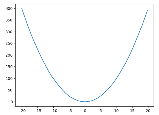
The mathematical solution will be to find the derivative, then solve the equation, $\frac{\partial f(x)}{\partial x} = 2x = 0$ , which gives the solution as x = 0. But what if you don’t know this and need to rely on a method which can reach the minimum of a function iteratively. That is what gradient descent does.

Gradient descent as the name suggests is like slowly descending down the mountain that is the loss function but in an iterative manner. We always take a small step in the opposite direction of the gradient. If the gradient is positive, we take a negative step and if the gradient is negative then we take a positive step.

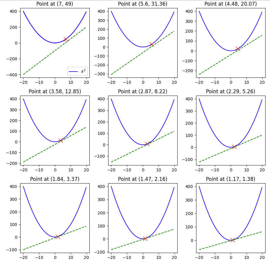
So in this example suppose we have to minimise $x^{2}$ and we start off with an initial value say 7. Then we we will update the value of x as –

x_new = x_old + (- $\frac{\partial f(x)}{\partial x}$ )*x_old*lr

where lr is the learning rate. Tuning this value is crucial is how fast we reach the minimum, or if we overshoot the minimum and never reach it.

Let’s take an example in python –
```
import matplotlib.pyplot as plt
import matplotlib.animation as animation
import numpy as np

def f(x):
    return x**2

def derivative(x):
    return 2*x

y = [f(x) for x in np.arange(-20,20,0.2)]
x = np.arange(-20,20,0.2)

plt.plot(x,y)
```
```
value = 7
lr = 0.1
derivatives = []
values = []
for i in range(9):
    values.append(value)
    derivatives.append(derivative(value))
    value = value - lr*derivative(value)

# List of points and derivatives
points = [(x,f(x)) for x in values]

# Create a 9x9 subplot grid
fig, axs = plt.subplots(3, 3, figsize=(9, 9))


# Plot the main plot (x^2) in the top-left subplot
axs[0, 0].plot(x, y, label='$x^2$', color='blue')
axs[0, 0].legend()

# Iterate over points and derivatives to create subplots
for i, (point_x, point_y) in enumerate(points):
    # Calculate the line passing through the point with the slope from the derivatives list
    slope = derivatives[i]
    line_y = x + slope * (x - point_x)

    axs[i//3, i%3].plot(x, y, color='blue')

    # Plot the point
    axs[i//3, i%3].plot(point_x, point_y, marker='x', markersize=10, color='red', label='Point')
    
    # Plot the line passing through the point with the specified slope
    axs[i//3, i%3].plot(x, line_y, linestyle='--', color='green', label=f'Slope = {slope}')

    # Set titles for subplots
    axs[i//3, i%3].set_title(f'Point at ({np.round(point_x,2)}, {np.round(point_y,2)})')

# Adjust layout for better visualization
plt.tight_layout()

# Show the plot
plt.show()
```
Here we see that with a learning rate of 0.1 and a starting value of 7 and in 9 steps we were able to reach 1.17, pretty close to the minimum of 0, but not quite so, if we change the lr to 0.3, let’s see what happens.

The minimum of 0 was reached within 9 steps.

But what happens if we make the lr 1 –

Here you can see that the value keeps oscillating between 7 and -7, and thus having a large learning rate also can be harmful when using ML models that use gradient descent.

Hopefully this example gave you a visual guide on how gradient descent works.
January 22, 2024