Tag: Machine Learning

  • Custom Objective Function in XGBoost

    In the previous post, we covered how you can create a custom loss function in Catboost, but you might be using catboost, so how can you create the same if you’re using Xgboost to train your models. In this post, I’ll walk over an example using the famous Titanic dataset, where we’ll recreate the LogLoss function and compare the results with the standard implementation in the library.

    First, we have to set up the data.

    import numpy as np 
    import seaborn as sns
    import pandas as pd
    import xgboost as xgb
    from sklearn.metrics import log_loss

    data = sns.load_dataset('titanic')

    Then some data cleaning and setting up the training dataset. The goal is not to get the best model but to demonstrate the custom loss function, so not much feature engineering is being done.

    data['embarked'].fillna('S', inplace = True)

    X,y = data[[c for c in data.columns if c not in \
    ['survived', 'alive', 'deck', 'embark_town']]], \
    data['survived']

    cat_columns = ['pclass', 'sex', 'sibsp', 'parch', 'embarked', 'class',
    'who', 'adult_male', 'alone']

    X = pd.get_dummies(X, columns=cat_columns, drop_first=True)

    Let’s say there was no loss function like logloss, then how would you define the logloss as an objective function.

    LogLoss = -1/N \sum({y_{i}log(\hat{y}) + (1-y_{i})log(1-\hat{y})})

    You’ll have to calculate the first and second derivative with respect to the \hat{y}

    \Large \frac{\partial LogLoss}{\partial \hat{y}} = -\frac{y_{i}}{\hat{y}} + \frac{1-y_{i}}{1-\hat{y}}

    \Large  \frac{\partial^2LogLoss }{\partial \hat{y}^2} = \frac{y_{i}}{\hat{y}^{2}} + \frac{1-y_{i}}{(1-\hat{y})^{2}}

    Now we will write these up as Python functions and create a function that returns the gradient and hessian (second derivative) values. In the xgboost library, the first value being passed is the predictions and the second is the training matrix.

    def log_loss_derivative(y_pred, dtrain ):
    y = dtrain.get_label()
    return (-y/y_pred) + ((1-y)/(1-y_pred))

    def log_loss_second_derivative(y_pred, dtrain):
    y = dtrain.get_label()
    return (y/np.power(y_pred,2)) + ((1-y)/np.power((1-y_pred),2))

    def custom_log_loss(predt, dtrain):
    y_pred = np.clip(predt, a_max=1-1e-5, a_min=1e-5)
    grad = log_loss_derivative(y_pred= y_pred, dtrain = dtrain)
    hess = log_loss_second_derivative(y_pred= y_pred, dtrain = dtrain)
    return grad, hess

    We clip the predictions to avoid division by zero errors. Now let’s train.

    import xgboost as xgb

    dtrain =xgb.DMatrix(data=X, label=y)

    model = xgb.train({'tree_method': 'hist', 'seed': 1994},
    dtrain=dtrain,
    num_boost_round=10,
    obj=custom_log_loss)

    log_loss(y_pred=np.clip(model.predict(dtrain), a_max=1, a_min=0), y_true=y)
    >>>0.24912

    Comparison with the standard implementation.

    clf = xgb.XGBClassifier(n_estimators = 10, **{'tree_method': 'hist', 'seed': 1994})
    clf.fit(X,y)

    log_loss(y_pred=np.clip(clf.predict_proba(X)[:,1], a_max=1, a_min=0), y_true=y)

    >>>0.2861

    As we can see the metrics are very close in our implementation of the LogLoss and the standard implementation. Of course, you should use the standard implementation when it’s available, but in case you want to use a custom loss function, you now know how to do so.
  • Creating a Custom Loss Function For Machine Learning Models

    While standard Machine Learning Libraries provide a vast array of loss functions out of the box, sometimes we need to create our own custom loss function. In this blog post, I’ll go over a simple example and create a custom loss function in Catboost.

    First we will create the data for training.

    # Importing libraries
    import numpy as np
    import pandas as pd
    from sklearn.metrics import mean_squared_error
    from catboost import CatBoostRegressor, Pool
    from sklearn.datasets import fetch_california_housing

    raw_data = fetch_california_housing()

    data = pd.concat([pd.DataFrame(raw_data['data'], columns=raw_data['feature_names']),
    pd.Series(raw_data['target'], name = 'target')], axis = 1)

    features = [i for i in data.columns.tolist() if i != 'target']

    Since the objective is not to create the best model possible, we won’t be doing any feature engineering. Let’s use catboost, and create a model using standard loss functions.

    model = CatBoostRegressor(loss_function='RMSE', n_estimators=100, eval_metric='RMSE')

    cb_pool = Pool(data=data[features], label=data['target'], feature_names=features)

    model.fit(cb_pool)

    predictions = model.predict(cb_pool)

    mean_squared_error(y_true=data['target'], y_pred=predictions)

    Upon evaluating the model we find that the mean squared error is 0.15. Definitely a model which is overfitting, but that’s not a concern for this tutorial.

    But what is you don’t want to use RMSE as a loss function, and instead want to use something like this –

    loss = \frac{\sum (y - \hat{y})^{4}}{n}

    Then how do you create a loss function in catboost?

    For this, you’ll need to calculate the first derivative and the second derivative of the loss function with respect to \hat{y}.

    Using the chain rule, the first derivative is

    \frac{\partial (y-\hat{y})^4}{\partial \hat{y}} = \frac{\partial (y-\hat{y})^4}{\partial (y-\hat{y})}*\frac{\partial y - \hat{y}}{\partial \hat{y}} = 4 * (y - \hat{y})^{3}* -1 = -4(y -\hat{y})^{3}

    And similarly using the chain rule, the second derivative comes out to be 12*(y-\hat{y})^2

    The catboost template for a custom objective is as follows –

    class UserDefinedObjective(object):
        def calc_ders_range(self, approxes, targets, weights):
            """
            Computes first and second derivative of the loss function 
            with respect to the predicted value for each object.
    
            Parameters
            ----------
            approxes : indexed container of floats
                Current predictions for each object.
    
            targets : indexed container of floats
                Target values you provided with the dataset.
    
            weight : float, optional (default=None)
                Instance weight.
    
            Returns
            -------
                der1 : list-like object of float
                der2 : list-like object of float
    
            """
            pass
    

    Using this temple, we can write the custom objective –

    class CustomLossObjective(object):
    def calc_ders_range(self, approxes, targets, weights):
    assert len(approxes) == len(targets)
    if weights is not None:
    assert len(weights) == len(approxes)

    result = []
    n = len(targets) # Number of samples

    for index in range(len(targets)):
    error = targets[index] - approxes[index]
    der1 = -4 * error**3
    der2 = 12 * error**2

    if weights is not None:
    der1 *= weights[index]
    der2 *= weights[index]

    result.append((der1, der2))
    return result

    Now let’s use this custom loss in our model

    model = CatBoostRegressor(loss_function=CustomLossObjective(), n_estimators=100, eval_metric='RMSE')
    model.fit(cb_pool)

    predictions = model.predict(cb_pool)
    mean_squared_error(y_true=data['target'], y_pred=predictions)

    Using this loss, we see that the mean squared error is 0.735, this is clearly inferior to using RMSE, but as mentioned before the objective of this blog post is not to build the best model but to showcase how one can create a custom loss objective in catboost.

  • Understanding Naive Bayes – A simple yet powerful ML Model Part 1 – Bayes Theorem

    Naive Bayes is often not given enough credit, people when learning about ML often directly start using XgBoost or Random Forest models. While these models are good and will often achieve the task, we should also know about Naive Bayes, a Bayesian ML model, which was once used in production by tech giants like Google.

    But before we deep dive into Naive Bayes, we’ve to learn about the Bayes theorem itself.

    P(A/B) = \frac{P(B/A)*P(A)}{P(B)}

    It may seem daunting, but at its core, the formula is very simple to understand, all it provides is a way to calculate the probability of A given B has already happened. It is equal to the probability of B given that A has already happened multiplied by the probability of A divided by the probability of B happening.

    You might be daunted by mathematical jargon such as posterior and priors, but if you think in these simple terms then it is a very simple formula.

    Let’s take an example, and suppose that we don’t know Bayes theorem.

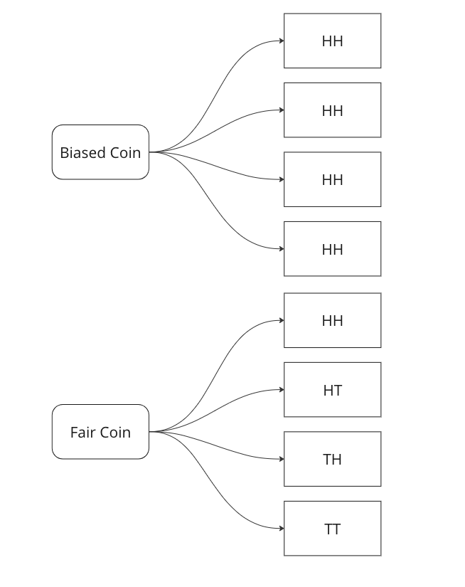
    We are told that a coin could be fair, or biased (always comes up heads). We observe two heads in a row and we have to find the probability that the coin being tossed is a fair coin.

    Graphing all outcomes of two coin tosses by both a fair and a biased coin. Now we know that two heads came in a row. So we update our sample space with this given information.

    Here we can see that we can only attribute 1 sample out of 5 to a fair coin, so P(fair coin/HH) = 1/5. In a similar way, we can say P(biased coin/HH) = 4/5 as we can attribute 4 out of 5 sample points to the biased coin.

    Let us see if we can arrive on the same answer by using the Bayes Formula.

    P(fair coin/HH) = \frac{P(HH/fair coin)*P(fair coin)}{P(HH)} = \frac{1/4*1/2}{1*1/2+1/2*1/4}=1/5

    Breaking down the calculations –

    1. P (HH/fair coin) = 1/4 – we saw above that in 1/4 cases a fair coin will give two heads
    2. P ( fair coin) = 1/2 – we know that a coin could be biased or fair, this is what is known as a prior, here it is equally likely that the coin could be biased or fair.
    3. P (HH) = 1/2*1 + 1/2*1/4 – This is where most of the confusion rises related to Bayes theorem. We have to calculate the probability of getting two heads, considering both scenarios. In the case of a biased coin, it will always gives head, so the probability is 1. There is also half a chance to select it, so we multiply it by 0.5. Similarly, we know 1/4 is the probability to get HH with a fair coin, and there is 0.5 probability to select it.

    In the next part we will see how we can use this to create a very basic classifier in Python.

  • Leave one out encoding – Encode your categorical variables to the target

    In case you want to use ML models on categorical variables, you’ve to encode them. The most common approach is one hot encoding. But what if you’ve too many categories and categorical variables, in this case, if you one hot encode, then you will end up with a very sparse matrix.

    Well there are ways you can tackle this, and I’ll be talking about one such way – Leave One Out Encoding.

    Leave-One-Out (LOO) is a cross-validation technique that involves splitting the data into training and test sets, where the test set contains a single sample, and the training set contains the remaining samples. LOO is performed for each sample in the dataset, and the model is trained and evaluated multiple times. In each split, you take the mean of the target for the category being encoded in train and add it to the test.

    Pros:

    1. Utilizes all available data: LOO ensures that each sample in the dataset is used as both a training and test instance. This maximizes the utilization of the available data and provides a more accurate estimate of model performance.
    2. Low bias: Since each training set contains all but one sample, the model is trained on almost the entire dataset. This reduces the bias introduced by other cross-validation techniques that use smaller training sets.
    3. Suitable for small datasets: LOO is particularly useful for small datasets where splitting the data into multiple folds might result in inadequate training data for model fitting.
    4. Unbiased estimator: LOO estimates tend to have lower bias compared to other cross-validation techniques, as the model is evaluated on independent samples.

    Cons:

    1. High computational cost: LOO requires training and evaluating the model as many times as there are samples in the dataset, making it computationally expensive, especially for large datasets.
    2. Variance and instability: LOO estimates can have high variance due to the high dependence between the training sets. Small changes in the data can lead to significant changes in the estimated performance. Thus, LOO estimates can be less stable than estimates obtained from other cross-validation methods.
    3. Overfitting risk: LOO can be prone to overfitting, as the model is trained on almost the entire dataset. This can result in overly optimistic performance estimates if the model is too complex or the dataset is noisy.
    4. Imbalanced class issues: If the dataset is imbalanced, LOO can lead to biased estimates, as each training set will typically contain a majority of samples from the majority class.

    Let’s walk through an examples.

    import pandas as pd
    import numpy as np
    from sklearn.model_selection import LeaveOneOut
    
    # Example data
    data = pd.DataFrame({
        'category': ['A', 'A', 'B', 'B', 'B', 'C', 'C', 'C'],
        'target': [1, 2, 3, 4, 5, 6, 7, 8]
    })
    
    # Create new column for leave-one-out encoded feature
    data['category_loo_encoded'] = np.nan
    

    Here we create a dummy data with a categorical variable and a numerical target.

    # Leave-One-Out Encoding
    loo = LeaveOneOut()
    
    for train_index, test_index in loo.split(data):
        X_train, X_test = data.iloc[train_index], data.iloc[test_index]
        
        # Calculate mean excluding the current row
        mean_target = X_train.loc[X_train['category'] == X_test['category'].values[0], 'target'].mean()
        
        # Assign leave-one-out encoded value
        data.loc[test_index, 'category_loo_encoded'] = mean_target
    
    # Display the result
    print(data)
    
    categorytargetcategory_loo_encoded
    A12
    A21
    B34.5
    B44
    B53.5
    C67.5
    C77
    C86.5

    There are also libraries that you can use which can help you with this. You can use category encoders. The advantage is that you can use parameters like sigma which adds noise and reduces overfitting.

    Here is the Python snippet on the same data.

    import category_encoders as ce
    # Create an instance of LeaveOneOutEncoder
    encoder = ce.LeaveOneOutEncoder(cols=['category'])
    
    # Perform leave-one-out encoding
    data_encoded = encoder.fit_transform(data['category'], data['target'])
    
    # Merge the encoded data with the original dataframe
    data = data.merge(data_encoded, how = 'left', left_index=True, right_index=True)
    
    # Display the result
    print(data)
    

    Here you can see we get the same result if we use category encoders as well.

    Thanks for reading and let me know in the comments in case you’ve any questions regarding Leave One Out Encoding.

  • MCC Score – The only ML metric you need

    The title might be a bit of a clickbait, but MCC (Matthews Correlation Coefficient) is a critical ML metric that every Data Scientist must know.

    Metrics like the F1 score focus on only one class and its performance, but if you want a balanced model then you should be optimising your model on MCC score rather than on Accuracy or F1-score.

    Let us take an example of –

    y_true = [1,1,1,1,0,0,1, 0,1]
    y_pred = [1,1,1,1,1,1,1, 0,0]

    If we calculate the F1-score then it is ~0.77, but the MCC score is ~0.19, meaning that even though the model is very good at classifying the positive class, it is not very good at the negative class.

    If we look at the formula for MCC –

    \[MCC = \frac{(TPxTN)-(FPxFN)}{\sqrt{(TP+FP)(TP+FN)(TN+FP)(TN+FN)}}\] https://www.hostmath.com/Math/MathJax.js?config=OK

    It should be clear that MCC gives equal focus on both TP and TN, since it is a correlation coefficient, its value ranges from -1 to 1.

  • K-Nearest Neighbour Algorithm Explained

    KNN (K-Nearest Neighbours) is a supervised learning algorithm which uses the nearest neighbours to classify a new data point.

    The tricky part is selecting the optimal k for the model.

    sklearn.neighbors.KNeighborsClassifier(n_neighbors=5*weights='uniform'algorithm='auto'leaf_size=30p=2metric='minkowski'metric_params=Nonen_jobs=None)

    As you can see the weights by default is uniform and the n_neighbours is by default 5. Large values of k smooth things, but a very small value of k will be unreliable and could be affected by outliers.

    You can pick the optimal value of the k by tuning the hyperparameter using GridSearchCV.

    Then there is the value of p, which is by 2, meaning that it uses the euclidean distance, you can set it to 1 to use Manhattan distance. This is the distance it uses to chose the nearest points for classification.

    Let’s code this in python-

    from sklearn.neighbors import KNeighborsClassifier
    from sklearn.datasets import load_iris
    from sklearn.model_selection import GridSearchCV
    
    X, y = load_iris()['data'], load_iris()['target']
    
    #defining the search grid
    param_grid = {'n_neighbors': np.arange(3,10,1),
                 'p': [1,2,3]}
    
    grid_search = GridSearchCV(estimator=KNeighborsClassifier(), param_grid=param_grid, scoring='accuracy', cv = 3)
    
    grid_search.fit(X,y)
    
    print(grid_search.best_params_)
    >>> {'n_neighbors': 4, 'p': 2}
    print(grid_search.best_score_)
    >>>0.9866666666666667
    

    Hope this post cleared how you can use KNN in your machine learning problems, and if you want me to write about any ML topic, just drop a comment below.