Tag: ML

  • Exploring Data Distribution Differences in Machine Learning: An Adversarial Approach

    Exploring Data Distribution Differences in Machine Learning: An Adversarial Approach

    First, a shout-out to Santiago, whose tweet inspired this post.

    In the realm of machine learning, ensuring that models perform well not only on training data but also on unseen test data is crucial. A common challenge that arises is the difference in data distribution between training and testing datasets, known as dataset shift. This discrepancy can significantly degrade the performance of a model when deployed in real-world scenarios. To tackle this issue, researchers and practitioners have developed various methods to detect and quantify differences in data distribution. One innovative approach is the adversarial method, which leverages concepts from adversarial training to assess and address these differences.

    Understanding Dataset Shift

    Before diving into the adversarial methods, it is essential to understand what dataset shift entails. Dataset shift occurs when the joint distribution of inputs and outputs differs between the training and testing phases. This shift can be categorised into several types, including covariate shift, prior probability shift, and concept shift, each affecting the model in different ways.

    • Covariate Shift: The distribution of input features changes between the training and testing datasets.
    • Prior Probability Shift: The distribution of the output variable changes.
    • Concept Shift: The relationship between the input features and the output variable changes.

    Detecting and correcting for these shifts is crucial for developing robust machine learning models.

    Adversarial Methods for Detecting Dataset Shift

    Adversarial methods for dataset shift detection are inspired by adversarial training in neural networks, where models are trained to be robust against intentionally crafted malicious input. Similarly, in dataset shift detection, these methods involve creating a scenario where a model tries to distinguish between training and testing data based on their data distributions.

    The way to do this is –

    1. Combine your train and test data.
    2. Create a new column, where you label training data as 1 and test data as 0.
    3. Train a classifier on this using your new column as the target.

    If the data in both train and test comes from the same distribution, the AUC will be close to 0.5, but if they are from different distributions, then the model will learn to differentiate the data points and the AUC will be close to 1.

    Example

    In this example, we will have training data as height and weight in metres and kilograms, and in the test data, we will have the same data but in centimetres and grams. Then if we train a simple logistic regression to learn on the dummy target, which is 1 on the training set and 0 on test data, given that we are not scaling the variables, the model should have an AUC close to 1.

    #Loading required libraries
    import numpy as np 
    import pandas as pd
    import seaborn as sns
    from sklearn.linear_model import LogisticRegression
    from sklearn.metrics import roc_auc_score
    from matplotlib import pyplot as plt
    

    Then we define our features for train and test

    # Set random seed for reproducibility
    np.random.seed(42)
    
    # Generate synthetic data
    # Training data (height in meters, weight in kilograms)
    train_height = np.random.normal(1.75, 0.1, 1000)  # Average height 1.75 meters
    train_weight = np.random.normal(70, 10, 1000)    # Average weight 70 kg
    
    # Test data (height in centimeters, weight in grams)
    test_height = train_height * 100  # Convert meters to centimeters
    test_weight = train_weight * 1000  # Convert kilograms to grams
    

    Once we’ve our features defined, all we need to do is create a training dataset, train our classifier and check the AUC score.

    # Combine data into feature matrices
    X_train = np.column_stack((train_height, train_weight))
    X_test = np.column_stack((test_height, test_weight))
    
    # Create labels: 1 for training data, 0 for test data
    y_train = np.ones(X_train.shape[0])
    y_test = np.zeros(X_test.shape[0])
    
    # Combine into a single dataset
    X = np.vstack((X_train, X_test))
    y = np.concatenate((y_train, y_test))
    
    # Train logistic regression model
    model = LogisticRegression()
    model.fit(X, y)
    
    # Predict probabilities for ROC AUC calculation
    y_pred_proba = model.predict_proba(X)[:, 1]
    
    # Calculate AUC
    auc = roc_auc_score(y, y_pred_proba)
    print(f"The AUC is: {auc:.2f}")


    The AUC here comes out to be 1.0 as expected. Since the train and test data comes from different distributions, the model was easily able to identify the difference in the distribution between train and test.

    Using this approach you can also easily test whether the train and test data come from the same distribution.

  • Cohen’s Kappa and its use in ML

    Suppose you’re building a classification model on an imbalanced dataset and you want to have other measures for your model other than accuracy, F1-score, and ROC-AUC curve, what else can you measure to be confident in your results. The answer is Cohen’s kappa.

    Cohen’s Kappa is a statistical measure that quantifies the level of agreement between two annotators or, in the context of ML, the agreement between the model’s predictions and the true labels. It accounts for the possibility of agreement occurring by chance, providing a more nuanced evaluation than traditional accuracy metrics.

    The Formula:
    The formula for Cohen’s Kappa is –

    \kappa = \frac{p_{0} - p_{e}}{1-p_{e}}

    Where p_{0} is the observed agreement between the model’s predictions and true labels and p_{e} is the expected agreement by chance.

    Let’s take an example to understand this better. A binary classification scenario where you’re building a spam email classifier. The task is to distinguish between spam and non-spam (ham) emails. We’ll use a simple logistic regression model for this example.

    from sklearn.model_selection import train_test_split
    from sklearn.feature_extraction.text import CountVectorizer
    from sklearn.linear_model import LogisticRegression
    from sklearn.metrics import accuracy_score, confusion_matrix, cohen_kappa_score

    # Sample data for spam and non-spam emails
    data = [
    ("Get rich quick! Claim your prize now!", "spam"),
    ("Meeting at 3 pm in the conference room.", "ham"),
    ("Exclusive offer for you!", "spam"),
    ("Reminder: Project deadline tomorrow.", "ham"),
    # ... more data ...
    ]

    # Split the data into training and testing sets
    X_train, X_test, y_train, y_test = train_test_split(
    [text for text, label in data],
    [label for text, label in data],
    test_size=0.2,
    random_state=42
    )

    # Vectorize the text data
    vectorizer = CountVectorizer()
    X_train_vec = vectorizer.fit_transform(X_train)
    X_test_vec = vectorizer.transform(X_test)

    # Train a logistic regression classifier
    classifier = LogisticRegression()
    classifier.fit(X_train_vec, y_train)

    # Make predictions on the test set
    y_pred = classifier.predict(X_test_vec)

    # Evaluate the model
    accuracy = accuracy_score(y_test, y_pred)
    conf_matrix = confusion_matrix(y_test, y_pred)
    kappa_score = cohen_kappa_score(y_test, y_pred)

    # Print the results
    print(f"Accuracy: {accuracy}")
    print(f"Confusion Matrix:\n{conf_matrix}")
    print(f"Cohen's Kappa: {kappa_score}")

    After this, you get a kappa of 1, which means that it’s an excellent model and there is no variability that can be attributed to chance. Be aware that this is an ideal scenario.

    Another scenario is that you get a score of 0, meaning that the model’s performance is no better than random chance, that is your features don’t capture any meaningful patterns in the data.

    In the context of model evaluation:

    Kappa scores closer to 1 indicate a high level of agreement and are generally considered desirable.

    Kappa scores around 0 or below suggest poor agreement, and the model’s predictions might not be reliable.

    It’s essential to interpret Cohen’s Kappa alongside other evaluation metrics, such as accuracy, precision, recall, and the confusion matrix, to comprehensively understand the model’s performance. Additionally, the interpretation of Kappa may vary depending on the specific problem and the level of difficulty in the classification task.

  • Understanding Naive Bayes – A simple yet powerful ML Model Part 1 – Bayes Theorem

    Naive Bayes is often not given enough credit, people when learning about ML often directly start using XgBoost or Random Forest models. While these models are good and will often achieve the task, we should also know about Naive Bayes, a Bayesian ML model, which was once used in production by tech giants like Google.

    But before we deep dive into Naive Bayes, we’ve to learn about the Bayes theorem itself.

    P(A/B) = \frac{P(B/A)*P(A)}{P(B)}

    It may seem daunting, but at its core, the formula is very simple to understand, all it provides is a way to calculate the probability of A given B has already happened. It is equal to the probability of B given that A has already happened multiplied by the probability of A divided by the probability of B happening.

    You might be daunted by mathematical jargon such as posterior and priors, but if you think in these simple terms then it is a very simple formula.

    Let’s take an example, and suppose that we don’t know Bayes theorem.

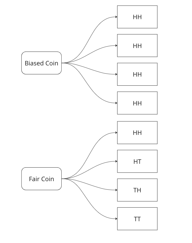
    We are told that a coin could be fair, or biased (always comes up heads). We observe two heads in a row and we have to find the probability that the coin being tossed is a fair coin.

    Graphing all outcomes of two coin tosses by both a fair and a biased coin. Now we know that two heads came in a row. So we update our sample space with this given information.

    Here we can see that we can only attribute 1 sample out of 5 to a fair coin, so P(fair coin/HH) = 1/5. In a similar way, we can say P(biased coin/HH) = 4/5 as we can attribute 4 out of 5 sample points to the biased coin.

    Let us see if we can arrive on the same answer by using the Bayes Formula.

    P(fair coin/HH) = \frac{P(HH/fair coin)*P(fair coin)}{P(HH)} = \frac{1/4*1/2}{1*1/2+1/2*1/4}=1/5

    Breaking down the calculations –

    1. P (HH/fair coin) = 1/4 – we saw above that in 1/4 cases a fair coin will give two heads
    2. P ( fair coin) = 1/2 – we know that a coin could be biased or fair, this is what is known as a prior, here it is equally likely that the coin could be biased or fair.
    3. P (HH) = 1/2*1 + 1/2*1/4 – This is where most of the confusion rises related to Bayes theorem. We have to calculate the probability of getting two heads, considering both scenarios. In the case of a biased coin, it will always gives head, so the probability is 1. There is also half a chance to select it, so we multiply it by 0.5. Similarly, we know 1/4 is the probability to get HH with a fair coin, and there is 0.5 probability to select it.

    In the next part we will see how we can use this to create a very basic classifier in Python.

  • Machine Learning In Production – Skew and Drift

    In this post we will go over a very important concept when it comes to Machine Learning models, especially when you deploy them in production.

    Drift: Drift, or concept drift, refers to the phenomenon where the statistical properties of the target variable or the input features change over time. In other words, the relationship between the input variables and the target variable is no longer stable. This can occur due to various reasons such as changes in the underlying data-generating process, changes in user behaviour, or changes in the environment. Concept drift can have a significant impact on the performance of machine learning models because they are trained on historical data that may no longer be representative of the current state. Models may need to be continuously monitored and updated to adapt to concept drift, or specialized techniques for handling concept drift, such as online learning or ensemble methods, can be employed.

    To measure this type of skew, you can use various statistical measures –

    1. Feature Comparison: Calculate summary statistics (such as mean, median and variance) for each feature in the training dataset and the production dataset. Compare these statistics to identify any significant differences. You can use measures like the Kolmogorov-Smirnov test or the Jensen-Shannon divergence to quantify the skew between the distributions.
    2. Domain Expertise: Consult with domain experts or stakeholders who are familiar with the data and understand the expected distribution of features. They can provide insights into potential skewness or changes in feature distributions that might be critical to consider.
    3. Monitoring and Drift Detection: Implement a monitoring system to track the distribution of features in the production environment continuously. There are various drift detection algorithms available, such as the Drift-Detection Method (DDM) or the Page-Hinkley Test. These methods analyze the incoming data over time and detect significant changes or shifts in the feature distributions.

    By combining these techniques, you can gain insights into the skewness between the training and production feature distributions. Detecting and addressing such skewness is crucial for maintaining the performance and reliability of machine learning models in real-world scenarios.

  • Leave one out encoding – Encode your categorical variables to the target

    In case you want to use ML models on categorical variables, you’ve to encode them. The most common approach is one hot encoding. But what if you’ve too many categories and categorical variables, in this case, if you one hot encode, then you will end up with a very sparse matrix.

    Well there are ways you can tackle this, and I’ll be talking about one such way – Leave One Out Encoding.

    Leave-One-Out (LOO) is a cross-validation technique that involves splitting the data into training and test sets, where the test set contains a single sample, and the training set contains the remaining samples. LOO is performed for each sample in the dataset, and the model is trained and evaluated multiple times. In each split, you take the mean of the target for the category being encoded in train and add it to the test.

    Pros:

    1. Utilizes all available data: LOO ensures that each sample in the dataset is used as both a training and test instance. This maximizes the utilization of the available data and provides a more accurate estimate of model performance.
    2. Low bias: Since each training set contains all but one sample, the model is trained on almost the entire dataset. This reduces the bias introduced by other cross-validation techniques that use smaller training sets.
    3. Suitable for small datasets: LOO is particularly useful for small datasets where splitting the data into multiple folds might result in inadequate training data for model fitting.
    4. Unbiased estimator: LOO estimates tend to have lower bias compared to other cross-validation techniques, as the model is evaluated on independent samples.

    Cons:

    1. High computational cost: LOO requires training and evaluating the model as many times as there are samples in the dataset, making it computationally expensive, especially for large datasets.
    2. Variance and instability: LOO estimates can have high variance due to the high dependence between the training sets. Small changes in the data can lead to significant changes in the estimated performance. Thus, LOO estimates can be less stable than estimates obtained from other cross-validation methods.
    3. Overfitting risk: LOO can be prone to overfitting, as the model is trained on almost the entire dataset. This can result in overly optimistic performance estimates if the model is too complex or the dataset is noisy.
    4. Imbalanced class issues: If the dataset is imbalanced, LOO can lead to biased estimates, as each training set will typically contain a majority of samples from the majority class.

    Let’s walk through an examples.

    import pandas as pd
    import numpy as np
    from sklearn.model_selection import LeaveOneOut
    
    # Example data
    data = pd.DataFrame({
        'category': ['A', 'A', 'B', 'B', 'B', 'C', 'C', 'C'],
        'target': [1, 2, 3, 4, 5, 6, 7, 8]
    })
    
    # Create new column for leave-one-out encoded feature
    data['category_loo_encoded'] = np.nan
    

    Here we create a dummy data with a categorical variable and a numerical target.

    # Leave-One-Out Encoding
    loo = LeaveOneOut()
    
    for train_index, test_index in loo.split(data):
        X_train, X_test = data.iloc[train_index], data.iloc[test_index]
        
        # Calculate mean excluding the current row
        mean_target = X_train.loc[X_train['category'] == X_test['category'].values[0], 'target'].mean()
        
        # Assign leave-one-out encoded value
        data.loc[test_index, 'category_loo_encoded'] = mean_target
    
    # Display the result
    print(data)
    
    categorytargetcategory_loo_encoded
    A12
    A21
    B34.5
    B44
    B53.5
    C67.5
    C77
    C86.5

    There are also libraries that you can use which can help you with this. You can use category encoders. The advantage is that you can use parameters like sigma which adds noise and reduces overfitting.

    Here is the Python snippet on the same data.

    import category_encoders as ce
    # Create an instance of LeaveOneOutEncoder
    encoder = ce.LeaveOneOutEncoder(cols=['category'])
    
    # Perform leave-one-out encoding
    data_encoded = encoder.fit_transform(data['category'], data['target'])
    
    # Merge the encoded data with the original dataframe
    data = data.merge(data_encoded, how = 'left', left_index=True, right_index=True)
    
    # Display the result
    print(data)
    

    Here you can see we get the same result if we use category encoders as well.

    Thanks for reading and let me know in the comments in case you’ve any questions regarding Leave One Out Encoding.

  • Balanced Log Loss, Metric for imbalanced classification problems

    We all know about LogLoss which is the main loss function when it comes to binary classification problems. The formula is given below –


    LogLoss = -\frac{1}{N} \sum_{i=1}^{N} \left( y_i \log(p_i) + (1 - y_i) \log(1 - p_i) \right)

    • (N) is the total number of samples.
    • (y_i) is the true label of sample (i) (0 or 1).
    • (p_i) is the predicted probability of sample (i) belonging to class 1.

    Imbalanced Log Loss:
    The imbalanced log loss accounts for class imbalance by introducing class weights. It can be defined as:


    ImbalancedLogLoss = -\frac{1}{N} \sum_{i=1}^{N} w_i \left( y_i \log(p_i) + (1 - y_i) \log(1 - p_i) \right)

    • (N) is the total number of samples.
    • (y_i) is the true label of sample (i) (0 or 1).
    • (p_i) is the predicted probability of sample (i) belonging to class 1.
    • (w_i) is the weight assigned to sample (i) based on its class label. For example, if class 0 has fewer samples than class 1, (w_i) can be set to the ratio of class 1 samples to class 0 samples.

    Here is the python code that you can call to evaluate in Catboost –

    class BalancedLogLoss:
        def get_final_error(self, error, weight):
            return error
    
        def is_max_optimal(self):
            return False
    
        def evaluate(self, approxes, target, weight):
            y_true = target.astype(int)
            y_pred = approxes[0].astype(float)
            
            y_pred = np.clip(y_pred, 1e-15, 1 - 1e-15)
            individual_loss = -(y_true * np.log(y_pred) + (1 - y_true) * np.log(1 - y_pred))
            
            class_weights = np.where(y_true == 1, np.sum(y_true == 0) / np.sum(y_true == 1), np.sum(y_true == 1) / np.sum(y_true == 0))
            weighted_loss = individual_loss * class_weights
            
            balanced_logloss = np.mean(weighted_loss)
            
            return balanced_logloss, 0.0

    Advantages of Imbalanced LogLoss –

    1. Handles Class Imbalance: The imbalanced log loss takes into account the class distribution and assigns appropriate weights to each class. This allows the model to effectively handle imbalanced datasets, where one class may have significantly fewer samples than the other. By assigning higher weights to the minority class, the model focuses more on correctly classifying the minority class, reducing the impact of class imbalance.
    2. Improves Model Performance: By incorporating class weights in the loss function, the imbalanced log loss guides the model to optimize its predictions specifically for imbalanced datasets. This can lead to improved model performance, as the model becomes more sensitive to the minority class and learns to make better predictions for both classes.
    3. Flexible Weighting Strategies: The imbalanced log loss allows flexibility in assigning weights to different classes. Various weighting strategies can be used based on the characteristics of the dataset and the specific problem at hand. For example, weights can be inversely proportional to class frequencies or can be set manually based on domain knowledge. This flexibility enables the model to adapt to different levels of class imbalance and prioritize the correct classification of the minority class accordingly.
    4. Evaluation Metric Consistency: When using the imbalanced log loss as both the training loss and evaluation metric, it ensures consistency in model optimization and evaluation. By optimizing the model to minimize the imbalanced log loss during training, the model’s performance is directly aligned with the evaluation metric, providing a fair assessment of the model’s effectiveness in handling class imbalance.

    In conclusion, if you have an imbalanced class problem, you can try this eval metric in your models as well.

    .

  • MSE vs MSLE, When to use what metric?

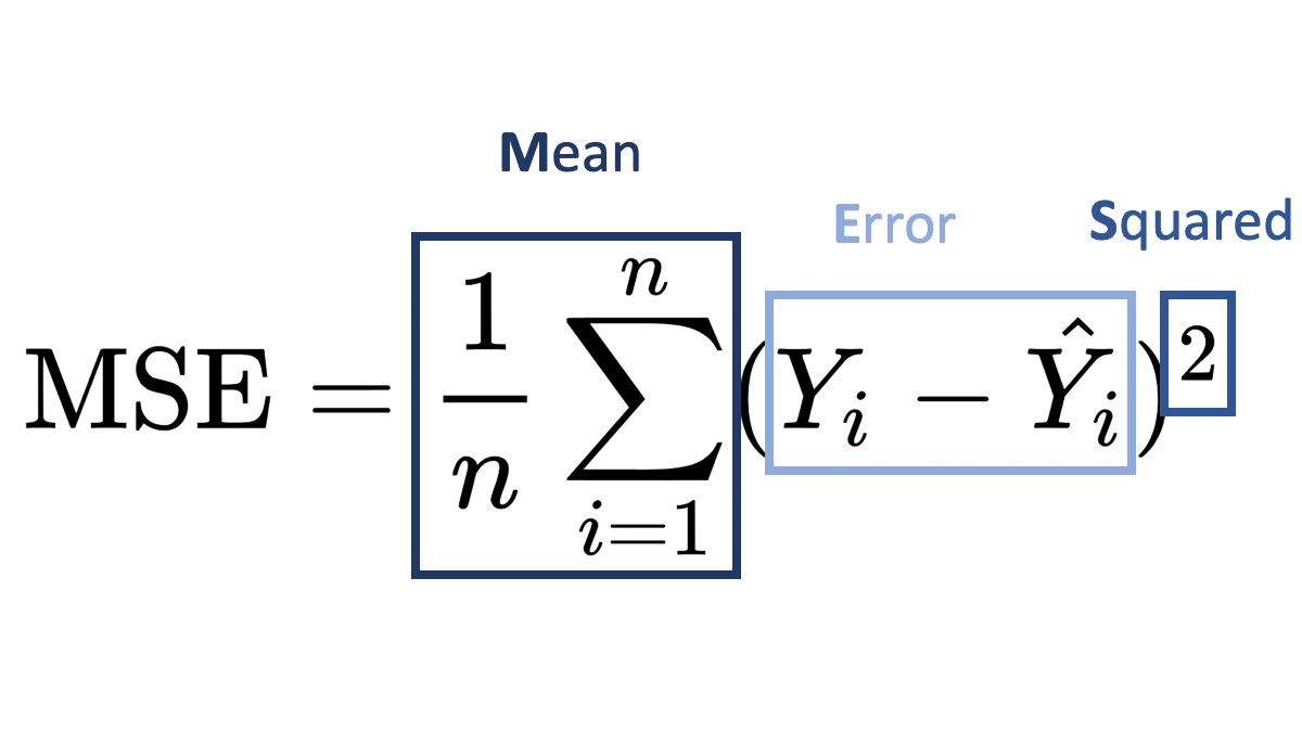
    MSLE (Mean Squared Logarithmic Error) and MSE (Mean Squared Error) are both loss functions that you can use in regression problems. But when should you use what metric?

    Mean Squared Error (MSE):

    It is useful when your target has a normal or normal-like distribution, as it is sensitive to outliers.

    An example is below –

    In this case using MSE as your loss function makes much more sense than MSLE.

    Mean Squared Logarithmic Error (MSLE):

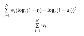
    • MSLE measures the average squared logarithmic difference between the predicted and actual values.
    • MSLE treats smaller errors as less significant than larger ones due to the logarithmic transformation.
    • It is less sensitive to outliers than MSE since the logarithmic transformation compresses the error values.

    An example where you can use MSLE –

    Here if you use MSE then due to the exponential nature of the target, it will be sensitive to outliers and MSLE is a better metric, remember that MSLE cannot be used for optimisation, it is only an evaluation metric.

    In general, the choice between MSLE and MSE depends on the nature of the problem, the distribution of errors, and the desired behavior of the model. It’s often a good idea to experiment with both and evaluate their performance using appropriate evaluation metrics before finalizing the choice.

  • K-Nearest Neighbour Algorithm Explained

    KNN (K-Nearest Neighbours) is a supervised learning algorithm which uses the nearest neighbours to classify a new data point.

    The tricky part is selecting the optimal k for the model.

    sklearn.neighbors.KNeighborsClassifier(n_neighbors=5*weights='uniform'algorithm='auto'leaf_size=30p=2metric='minkowski'metric_params=Nonen_jobs=None)

    As you can see the weights by default is uniform and the n_neighbours is by default 5. Large values of k smooth things, but a very small value of k will be unreliable and could be affected by outliers.

    You can pick the optimal value of the k by tuning the hyperparameter using GridSearchCV.

    Then there is the value of p, which is by 2, meaning that it uses the euclidean distance, you can set it to 1 to use Manhattan distance. This is the distance it uses to chose the nearest points for classification.

    Let’s code this in python-

    from sklearn.neighbors import KNeighborsClassifier
    from sklearn.datasets import load_iris
    from sklearn.model_selection import GridSearchCV
    
    X, y = load_iris()['data'], load_iris()['target']
    
    #defining the search grid
    param_grid = {'n_neighbors': np.arange(3,10,1),
                 'p': [1,2,3]}
    
    grid_search = GridSearchCV(estimator=KNeighborsClassifier(), param_grid=param_grid, scoring='accuracy', cv = 3)
    
    grid_search.fit(X,y)
    
    print(grid_search.best_params_)
    >>> {'n_neighbors': 4, 'p': 2}
    print(grid_search.best_score_)
    >>>0.9866666666666667
    

    Hope this post cleared how you can use KNN in your machine learning problems, and if you want me to write about any ML topic, just drop a comment below.

  • ML Metrics | Top N Accuracy Explained

    This metric is usually used in multiclass classification problems.
    Each multiclass model gives a probability score for all the classes it is being trained on, but often you take the highest one, by using np.argmax but what if you took the top n classes and gave credit to the model if it got right in one of the n predictions.
    That is what is top n accuracy, it gives the model more chances to be right.

    Lets take an example.

    Suppose you built a model that predicts 3 classes and you want to find the top 2 accuracy of your model.
    Then you would pass the prediction array to the model and the true values and if the correct prediction is in the top 2 then you give it credit for being right.

    import numpy as np
    from sklearn.metrics import top_k_accuracy_score
    y_true = [0,1,1,2,2]
    y_pred = [[0.25, 0.2,0.3], #Here 0 is in the top 2
              [0.3, 0.35, 0.5], #Here 1 is in the top 2
              [0.2,0.4, 0.45], #Here 1 is in the top 2
              [0.5, 0.1, 0.2], #Here 2 is in the top 2
              [0.1, 0.4, 0.2]] #Here 2 is in the top 2
    top_k_accuracy_score(y_true, y_pred, k=2)
    

    It is 1.0, because the correct class was always in our top 2 prediction, actually, if you notice then it was always the second prediction of our model, so if we take regular accuracy or set the value k = 1 in top_k_accuracy_score(y_true, y_pred, k=2), the answer is 0.

    Hopefully, this explains what top N accuracy is, and if you want me to cover any ML topic, write in the comments below. Thanks for reading.