Here are the 5 essential hyper-parameters that you should be always tuning when building any boosting model, whether you’re using XgBoost, LightGBM or even CatBoost.
n_estimators – It is not the number of trees that the boosting algorithm will grow, but as the name suggests, the number of times gradient boosting will occur, so if you are using a tree-based boosting algorithm, then if you make this number 5, then each round of boosting fits a single tree to the negative gradient of some loss function.
max_depth – The depth of each tree, pretty simple, the higher this number, the stronger each learner is in the model and the more your model can overfit. So pretty important to tune.
learning_rate – Again a very important param, the higher it is the faster your algorithm will converge to the local minima, but too high and it might overshoot the minima, too low and it might never reach the minima.
subsample – Sample of the training data to be used in each boosting round, if you use 0.5, then xgboost will randomly sample half your training data in each boosting iteration before growing the tree. Important if you want to control overfitting.
colsample_bytree – Fraction of columns to use when growing a tree, again if set to 0.5, xgboost will randomly sample half of your features to grow the tree in each boosting round. Again very important to control overfitting.
In another post I’ll be going over another 5 essential hyper-parameters that you should be tuning.
In this series of posts, I’ll be covering how to approach time series forecasting in python in detail. We will start with the basics and build on top of it. All posts will contain a practice example attached as a GitHub Gist. You can either read the post or watch the explainer Youtube video below.
# Loading Libraries
import numpy as np
import pandas as pd
import seaborn as sns
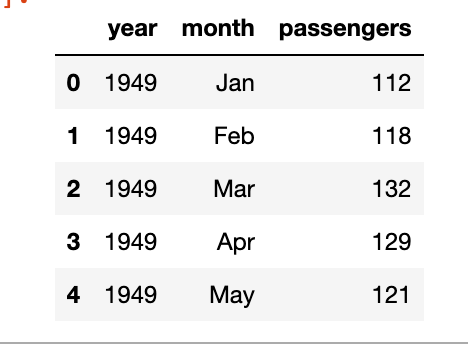
We will be using a simple linear regression to predict the outcome of the number of flights in the month of May. The data is taken from seaborn datasets.
As you can see we’ve the year, the month and the number of passengers, as a dummy example we will focus on the number of passengers in the month of May, below is the plot of year vs passengers.
We can clearly see a pattern here and can build a simple linear regression model to predict the number of passengers in the month of May in future years. The model will be like y = slope * feature + intercept. The feature, in this case, will be the number of passengers but shifted by 1 year. Meaning the number of passengers in the year 1949 will be the feature for the year 1950 and so on.
We can see that the p-value of the feature is significant, the intercept is not so significant, and the R-squared value is 0.97 which is very good. Of course, this is a dummy example so the values will be good.
df['prediction'] = df['lag_1']*m + b
sns.lineplot(x='year', y='value', hue='variable',
             data=pd.melt(df, ['year']))
The Unicorn Project is the successor to The Phoenix Project, written by Gene Kim. It’s a successor and not a sequel as you don’t need to read The Phoenix Project before reading this book. It introduces new characters in the story of Parts Unlimited. The story is told from the viewpoint of Maxine, a senior lead developer.
The story starts with Maxine being exiles to work on The Phoenix Project and there she is crippled by the way things work and she cannot even get her dev environment at the beginning and is stuck in a cycle of approvals and tickets. The book goes over familiar situations that developers and even Data Scientists or ML Engineers often come across where lack of proper infrastructure or planning of services hinder our development and delay things for weeks which can be done in hours had the design or processes been designed in a better manner.
It’s not just a story of the issues we face in our daily work life but also about overcoming those challenges, what best practices to follow and how leaders inspire and handle pressure situations. The novel coveys some essential skills that everyone should aspire to achieve in a fun story about the struggles of working on the behemoth that is The Phoenix Project and how Maxine with her friends of rebels creates The Unicorn Project. It is a story of failure and success, of how even a senior lead developer can learn from her peers and grow despite the hurdles imposed on her by the organisation. It also showcases how it is very important to know how your customers are using the product you’re building and whether the features you are introducing will help them or not.
The Unicorn Project is a must read for anyone working in the tech industry, whether you’re a software engineer, a DevOps or a Machine Learning Engineer, this book is for everyone.
So today I was participating in this Kaggle competition and the data had too many categorical variables. One way to build a model with too many categorical variables is to use a model like Catboost and let it deal with encoding categorical variables. But I wanted to ensemble my results with an Xgboost model, so I had to encode them. Using the weight of evidence encoding, I got a solution which was a top 10 solution when submitted. I have made the notebook public, you can go here and see it.
So what is weight of evidence ?
To put it simply –
I’ve gone through an example explaining the weight of evidence in the youtube video below.
One often thinks that you can use deep learning for classification problems like text or image classification, or for similar tasks like segmentation, language models etc. But you can also do simple linear regression with deep learning libraries. I’ve also attached the GitHub Gist in case you want to explore the working notebook.
In this post I’ll go over the model, it’s explanation on how can you do linear regression with keras.
In Keras, it can be implemented using the Sequential model and the Dense layer. Here’s an example of how to implement linear regression with Keras:
First we take a toy regression problem from scikit-learn datasets.
from sklearn.datasets import load_diabetes
from sklearn.model_selection import train_test_split

X,y = load_diabetes(return_X_y=True)

X_train, X_test, y_train, y_test = train_test_split(X,y, train_size=0.8)
Now we will need to define the model using Keras. That is actually very simple, you just have to take one sequential model with a Dense layer. The activation for this layer will be linear as we’re building a linear model and the loss will be mean squared error.
import numpy as np
from keras.models import Sequential
from keras.layers import Dense

# define the model
model = Sequential()
model.add(Dense(units=1, activation='linear'))
# compile the model
model.compile(optimizer='sgd', loss='mean_squared_error', metrics = ['mae'])

#fit the model
model.fit(x=X_train, y=y_train, validation_data=(X_test,y_test),
          epochs=100, batch_size=128)
Thats then all that is left is to call model.predict(X_test).
In this post, we will go over the complete decision tree theory and also build a very basic decision tree using information gain from scratch.
The below jupyter notebook as a Github Gist shows all the explanations and steps, including how to calculate Gini, Information gain and building a decision tree using the information gain you calculate.
You can also watch the video explainer here on youtube.
Random projection is another dimensionality reduction algorithm like PCA, as the name suggests, the basic idea behind Random Projection is to map the original high-dimensional data onto a lower-dimensional space while preserving as much of the pairwise distances between the data points as possible. This is done by generating a random matrix of size (n x k) where n is the dimensionality of the original data and k is the desired dimensionality of the reduced data.
If we have a matrix M of dimension and another matrix R of dimension whose columns are representing random directions, the random projection of M is then calculated as
The idea behind random projection is similar to PCA, but in PCA we first compute the eigenvalues, here we project the vector on random directions without any complex computations.
The random matrix used for the projection can be generated in a variety of ways. One popular method is the Johnson-Lindenstrauss lemma, which states that the pairwise distances between the points in the original space can be approximately preserved if the dimensionality of the lower-dimensional space is chosen to be logarithmic in the number of data points. Another popular method is the use of random gaussian matrix.
The Gaussian random projection reduces the dimensionality by projecting the original input space on a randomly generated matrix where components are drawn from the following distribution .
Why use Random Projection in place of PCA ?
Random Projection is often used in large-scale data analysis and machine learning applications where computational resources are limited and the dimensionality of the data is too high. In such cases, calculating PCA is often too time-consuming and computationally expensive. Additionally, Random Projection is less sensitive to the presence of noise and outliers in the data compared to PCA.
While the questions that you may be asked in a data science interview can vary a lot depending on the job description and the skillsets the organisation is looking for, there are a few questions that are often asked and as a candidate, you should know the answer to these.
Here in this post I’ll try to cover 10 such questions that you should know –
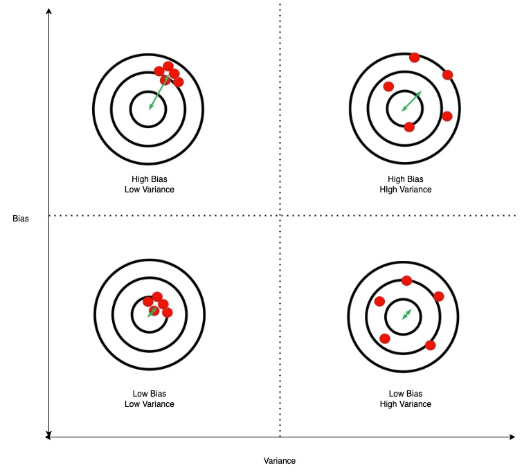
1. What is Bias-Variance Trade-off?
Bias in very simple terms is the error of your ML model. Variance is the difference in the evaluation metric in the train set and the test set that your model achieves. With any machine learning model, you try to reduce both bias and variance. The bias-variance trade-off is as you reduce bias, variance usually increases. So you try to select the ML model which has the lowest bias and variance. The below diagram should explain bias and variance.
2. In multiple linear regression if you keep adding dependent variables, the coefficient of determination (R-squared value) keeps going up, how do you then measure whether the model is improving or not?
In case of multiple linear regression, in addition to the you also calculate the adjusted r2, , which adjusts for the number of variables in the model and penalizes models with an excessive number of variables.
You should stop adding dependent variables when the adjusted r2 values starts to worsen
3. How does Random Forest reduce variance?
The main idea behind the Random Forest algorithm is to use low-bias decision trees and aggregate their results to reduce variance. Since each tree is grown from a bagged sample and also the features are bagged, meaning that each tree is grown from a different subset of features, thus the trees are not correlated and hence their combined results lead to lower variance than a single decision tree with low bias and high variance.
4. What are the support vectors in support vector machine (SVM)?
The support vectors are the data points that are used to define the decision boundary, or hyperplane, in an SVM. They are the key data points that determine the position of the decision boundary, and any change in these support vectors will result in a change in the decision boundary.
5. What is cross-validation and how is it used to evaluate a model’s performance?
Cross-validation involves dividing the available data into two sets: a training set and a validation set. The model is trained on the training set, and its performance is evaluated on the validation set. This process is repeated multiple times with different partitions of the data, and the performance measure is averaged across all iterations. This gives a more robust estimation of the model’s performance than a single train test split can do.
There are different types of cross-validation methods like k-fold cross-validation, in which the data is divided into k-folds, and the model is trained on k-1 folds and tested on the remaining fold. This process is repeated k times, and the performance measure is averaged across all iterations. Another one is Leave one out Cross-validation(LOOCV), in this method we use n-1 observations for training and the last one for testing. There is also a time-series cross-validation where the model is trained till time t and tested for a time after t. The window of training time keeps expanding after each iteration, it is also called expanding window cross-validation for time series.
I’ll be posting more Data Science questions on the blog so keep following for updates.
I was going through Kaggle competitions when this competition caught my eye, especially the evaluation metric for it. Now the usual metrics for forecasting or regression problems are either or , but sMAPE is different.
SMAPE (Symmetric Mean Absolute Percentage Error) is a metric that is used to evaluate the accuracy of a forecast model. It is calculated as the average of the absolute percentage differences between the forecasted and actual values, with the percentage computed using the actual value as the base. Mathematically, it can be expressed as:
So when to use which metric ?
RMSE – When you want to penalize large outlier errors in your prediction model, RMSE is the metric of choice as it penalizes large errors more than smaller ones.
MAPE – All errors have to be treated equally, so in those cases MAPE makes sense to use
sMAPE – is typically used when the forecasted values and the actual values are both positive, and when the forecasts and actuals are of similar magnitudes. It is symmetric in that it treats over-forecasting and under-forecasting the same.
It is important to note that in both MAPE and sMAPE, values of 0 are not allowed for both actual and forecast values as it would result in division by zero error.
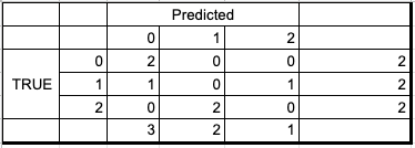
In this post, I’ll go over macro and micro averages, namely precision, and recall.
What is macro and micro averages ?
A macro takes the measurement independently of each class and then takes the average, thus giving equal weight to each class whereas a micro will take the class imbalances into account when computing the average.
When to use macro vs micro averages ?
If you suspect class imbalances to be there, then micro average should be preferred to macro.


 and another matrix R of dimension
  whose columns are representing random directions, the random projection of M is then calculated as
 .
.
 you also calculate the adjusted r2,
  , which adjusts for the number of variables in the model and penalizes models with an excessive number of variables.
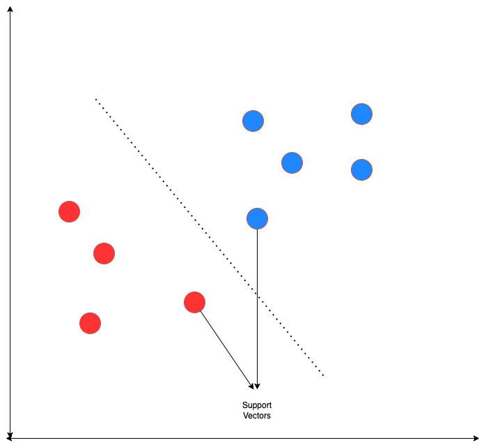
 or
or  , but sMAPE is different.