I often find people who are just starting out using pandas struggling to grasp when they should be using axis=0 and axis=1. While I go into a lot more detail with examples in the Youtube video above, you should keep this in mind.
When you use axis=0, pandas only looks at the value being passed, but when you use axis=1, by default it assumes a pandas Series being passed, so it looks for the index. So when you write a function which references multiple columns and use apply, use axis=1 and remember that it considers each row as a pandas Series, with the column names in the index.
Suppose you want to calculate aggregated count features and add them to your data frame as a feature. What you would typically do is, create a grouped data frame and then do a join. What if you can do all that in just one single line of code. Here you can use the transform functionality in pandas.
import numpy as np
import pandas as pd
import seaborn as sns
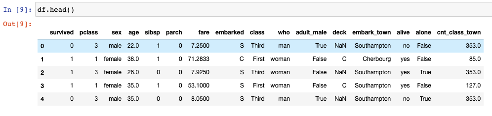
df = sns.load_dataset('titanic')
df.head()
Using df['cnt_class_town'] = df.groupby(['class', 'embark_town']).transform('size') we can directly get our desired feature in the data frame.
Again, if you want to create any sort of binned features based on the quantiles, usually first you would create a function and then use pandas apply to add that bucket to your data. Here again, you can directly use qcut functionality from pandas, pandas.qcut(x, q, labels=None, retbins=False, precision=3, duplicates='raise') to create the buckets in just one line of code.
Let’s take an example where we want to bin the age column into 4 categories, we can do so by running this one line of code –
In Part 1 of this series, we covered how you can use lag features and simple linear regression models to do time series forecasting, but that is very simple and you cannot capture trends using that model which is non-linear.
So we will be discussing different types of moving averages you can calculate in python and how they are helpful.
Simple Moving Average
# Loading Libraries
import numpy as np
import pandas as pd
import seaborn as sns
sns.set_theme()
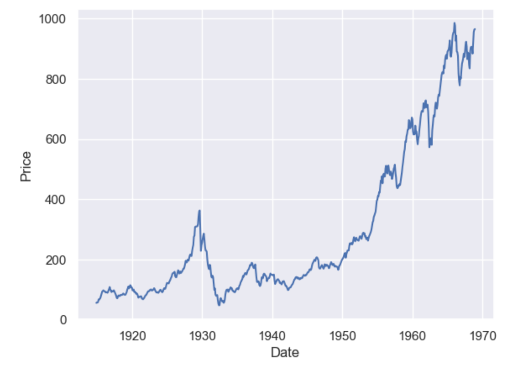
#Using the available dowjones data in seaborn
dowjones = sns.load_dataset("dowjones")
dowjones.head()
sns.lineplot(data=dowjones, x="Date", y="Price")
A simple moving average (SMA) calculates the average of a selected range of values, by the number of periods in that range. The most typical moving averages are 30-day, 50-day, 100-day and 365 day moving averages. Moving averages are nice cause they can determine trends while ignoring short-term fluctuations. One can calculate the sma by simply using
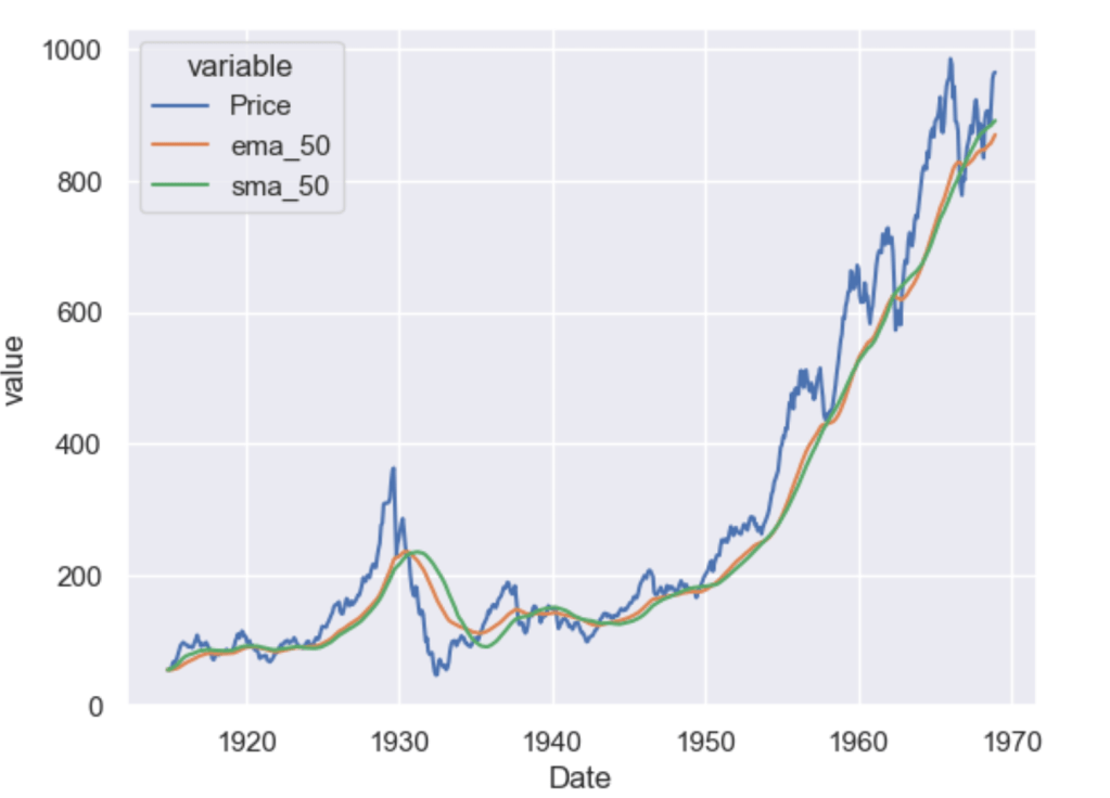
As you can see the higher the value of the window, the lesser it is affected by short-term fluctuations and it captures long-term trends in the data. Simple Moving Averages are often used by traders in the stock market for technical analysis.
Exponential Moving Average
Simple moving averages are nice, but they give equal weightage to each of the data points, what if you wanted an average that will give higher weight to more recent points and lesser to points in the past. In that case, what you want is to compute the exponential moving average (EMA).
As you can see the ema_50 follows the Price chart more closely than the sma_50 and is more sensitive to the recent data points.
Which moving average you should use as a feature of your forecasting model is a question mostly dependent on the use case. However, you will often use some kind of moving average as a feature or to visualise long-term or short-term trends in your data.
In Part 3 we explore trends and seasonality and how can you identify them in your data.
How to transform your data to generate insights is one of the most essential skills a Data Scientist can have. Knowing state-of-the-art models will be of no use if you cannot transform your data with ease. Pandas is a data manipulation library in python that everyone knows. It is so ubiquitous that all of us starting off in Data Science start our notebooks with import pandas as pd.
In this post, we will go over some pandas skills that many people either don’t know, don’t use or find difficult to understand.
As usual, you can either read the post or watch the Youtube video below.
We will be using the flights data from seaborn as an example to go over.
import pandas as pd
import numpy as np
import seaborn as sns
flights = sns.load_dataset('flights')
flights.head()
Pivot and Pivot Table
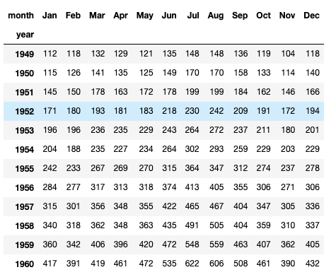
Now suppose that you want to create a table which had year as rows and month as columns and the passengers as values, then you will use pivot. Here is the pivot function from the official documentation of pandas – DataFrame.pivot(*, index=None, columns=None, values=None)
In this particular example, you’ll use year as index, month as columns and passengers in values.
Now the most important question is why there is pivot and a pivot_table in pandas. The reason is that pivot only reshapes the data, it does not support data aggregation, for data aggregation you will have to use pivot_table.
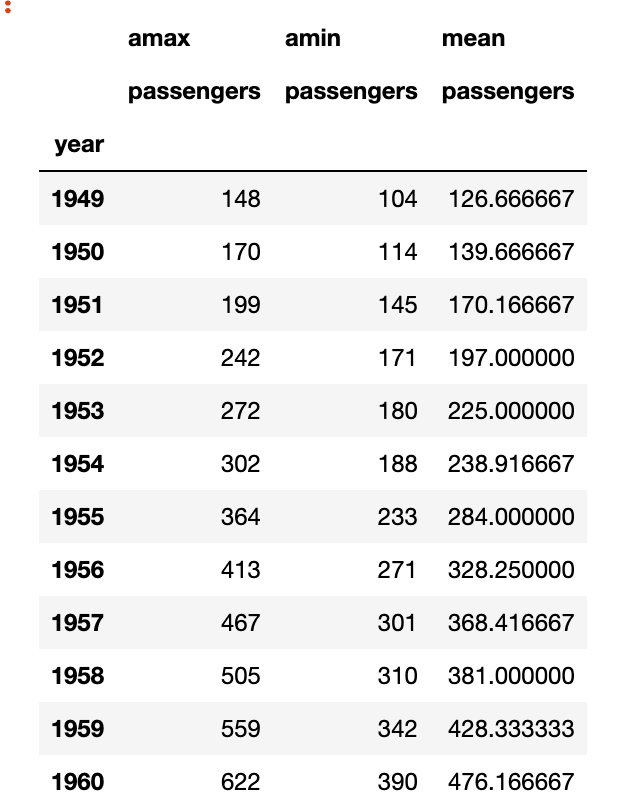
Now suppose I wanted to create a table which will show me for every year, what was the maximum, minimum and mean number of passengers, then there are two ways I can do it, I can either use groupby or I can use pivot_table. Here is the official documentation from pandas for pivot_table. Note: You can pass multiple aggregation functions.
And we wanted to return to the flights data form, then melt can be thought of as the unpivot of pandas. To return to the original form you simply have to –
Here we don’t use an id_var as there is None, we add ignore_index as False as we want to return the index which has the year in it and we call the value_name as passengers.
As a recap, remember that pivot makes long-form data into wide-form and melt takes wide-form data and converts it into long-form data
So where is Cast in Pandas?
People who have used R as a programming language often ask where is the cast functionality in pandas, the pivot_table we saw earlier is pandas’s answer to the cast functionality in Python.
Sometimes, coding questions are also part of data science interviews, so here is the solution to LeetCode #11 – the container with the most water problem.
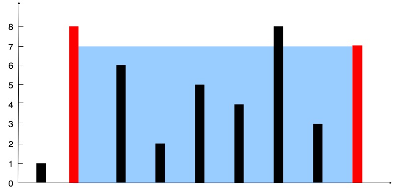
The problem is very straightforward, you’re given a list with n integers, each representing the height of a tower, you’ve to find the maximum area that can be formed with these heights and the x-axis represents the index distance between the integers with a twist that since it represents a block containing water, you’ve to take the min of the two heights as the water has to contained within the towers.
For example, if the list of given heights is h = [1,1,4,5,10,1], the maximum area that can be formed will be 8. It will be between the tower with heights 4 and 10, with an index distance of 2. So the area will be min(4,10)*2 = 8.
Coming to the solution, the easiest solution will be to compare each combination of two tower heights, and return the maximum area that can be formed. This will have a time complexity of
def maxArea(height: List[int]) -> int:
        max_vol = 0
        for i in range(len(height)):
            for j in range(1,len(height)):
                if j<=i:
                    continue
                else:
                    vol = min(height[i], height[j])*(j-i)
                    max_vol = max(max_vol, vol)
        return max_vol
Although the above solution will pass the sample test cases, it will eventually return Time Limit Exceeded as it is a very brute force solution, as it compares almost every possible combination. You can be a bit more clever in your approach and solve this problem in time complexity.
The trick is using pointers, one for left and one for right, starting with the largest width and then storing the max area. Move the left pointer right if you encounter a higher tower in the left otherwise move the right pointer towards the left, and repeat till both pointers meet. In this way, you’ve traversed the list only once.
def maxArea(height: List[int]) -> int:
        l,r = 0,len(height) - 1
        max_vol = -1
        while l < r:
            #Calculating the shorter height of the two
            shorter_height = min(height[l], height[r])
            width = r-l
            vol = shorter_height * width
            max_vol = max(vol, max_vol)
            if height[l] < height[r]:
                l+=1
            else:
                r-=1
        return max_vol
Taking an example, if input is [1,4,5,7,4,1], then.
Step
l
r
width
min height
area
max area
1
0
5
5
1
5
5
2
0
4
4
1
4
5
3
1
4
3
4
12
12
4
1
3
2
4
8
12
5
2
3
1
5
5
12
The loop will exit after step 5 as in step 6 l = r = 3, and we get the max area as 12.


 time complexity.