While standard Machine Learning Libraries provide a vast array of loss functions out of the box, sometimes we need to create our own custom loss function. In this blog post, I’ll go over a simple example and create a custom loss function in Catboost.
First we will create the data for training.
# Importing libraries
import numpy as np
import pandas as pd
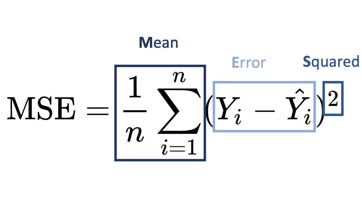
from sklearn.metrics import mean_squared_error
from catboost import CatBoostRegressor, Pool
from sklearn.datasets import fetch_california_housing
raw_data = fetch_california_housing()
data = pd.concat([pd.DataFrame(raw_data['data'], columns=raw_data['feature_names']),
pd.Series(raw_data['target'], name = 'target')], axis = 1)
features = [i for i in data.columns.tolist() if i != 'target']Since the objective is not to create the best model possible, we won’t be doing any feature engineering. Let’s use catboost, and create a model using standard loss functions.
model = CatBoostRegressor(loss_function='RMSE', n_estimators=100, eval_metric='RMSE')

cb_pool = Pool(data=data[features], label=data['target'], feature_names=features)

model.fit(cb_pool)

predictions = model.predict(cb_pool)

mean_squared_error(y_true=data['target'], y_pred=predictions)
Upon evaluating the model we find that the mean squared error is 0.15. Definitely a model which is overfitting, but that’s not a concern for this tutorial.
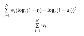
But what is you don’t want to use RMSE as a loss function, and instead want to use something like this –

Then how do you create a loss function in catboost?
For this, you’ll need to calculate the first derivative and the second derivative of the loss function with respect to 
Using the chain rule, the first derivative is

And similarly using the chain rule, the second derivative comes out to be

The catboost template for a custom objective is as follows –
class UserDefinedObjective(object):
    def calc_ders_range(self, approxes, targets, weights):
        """
        Computes first and second derivative of the loss function
        with respect to the predicted value for each object.

        Parameters
        ----------
        approxes : indexed container of floats
            Current predictions for each object.

        targets : indexed container of floats
            Target values you provided with the dataset.

        weight : float, optional (default=None)
            Instance weight.

        Returns
        -------
            der1 : list-like object of float
            der2 : list-like object of float

        """
        pass
Using this temple, we can write the custom objective –
class CustomLossObjective(object):
    def calc_ders_range(self, approxes, targets, weights):
        assert len(approxes) == len(targets)
        if weights is not None:
            assert len(weights) == len(approxes)

        result = []
        n = len(targets)  # Number of samples

        for index in range(len(targets)):
            error = targets[index] - approxes[index]
            der1 = -4 * error**3
            der2 = 12 * error**2

            if weights is not None:
                der1 *= weights[index]
                der2 *= weights[index]

            result.append((der1, der2))
        return result
Now let’s use this custom loss in our model
model = CatBoostRegressor(loss_function=CustomLossObjective(), n_estimators=100, eval_metric='RMSE')
model.fit(cb_pool)

predictions = model.predict(cb_pool)
mean_squared_error(y_true=data['target'], y_pred=predictions)
Using this loss, we see that the mean squared error is 0.735, this is clearly inferior to using RMSE, but as mentioned before the objective of this blog post is not to build the best model but to showcase how one can create a custom loss objective in catboost.